APIs, time-series, and weather Data
Course Schedule
Final Projects
- Only 9 folks have published their sites…
- Start moving your project proposal content into your website
- Title
- Introduction
- etc…
Resource Presentations
Case Study Presentations - Let’s pick a winner!
Next Week’s Case Study
API
Application Programming Interface
- Imagine I wanted to work with Wikipedia content…
Manually processing information from the web
- Browse to page,
File->Save As, repeat. - Deal with ugly html stuff…
<!DOCTYPE html>
<html>
<head>
  <meta charset="utf-8">
  <meta name="generator" content="pandoc">
  <title>APIs, time-series, and weather Data</title>
  <meta name="apple-mobile-web-app-capable" content="yes">
  <meta name="apple-mobile-web-app-status-bar-style" content="black-translucent">
  <meta name="viewport" content="width=device-width, initial-scale=1.0, maximum-scale=1.0, user-scalable=no, minimal-ui">
<link rel="stylesheet" href="externals/reveal.js-3.3.0.1/css/reveal.css"/>APIs allow direct (and often custom) sharing of data
c1=content$parse$wikitext%>%
  str_split(boundary("sentence"),simplify = T)%>%
  str_replace_all("'","")%>%
  str_replace_all("\\[|\\]","")
# results:
cat(c1[5:6])
##
## An application programming interface (API) is a connection between computers or between computer programs.Many data providers now have APIs
- Government Demographic data (census, etc.)
- Government Environmental data
- Google, Twitter, etc.
ROpenSci
Pros & Cons
Pros
- Get the data you want, when you want it
- Automatic updates - just re-run the request
Cons
- Dependent on real-time access
- APIs, permissions, etc. can change and break code
Generic API Access
- Provide R with a URL to request information
- The API sends you back a response
- JavaScript Object Notation (JSON)
- Extensible Markup Language (XML).
Endpoints
The URL you will request information from.
- Data.gov API: https://www.data.gov/developers/apis
- Github API: https://api.github.com
- U.S. Census API: http://api.census.gov
Some R Packages for specific APIs
Census data
library(tidycensus)

net_migration <- get_estimates(geography = "county",
                               variables = "RNETMIG",
                               geometry = TRUE) %>%
                               tigris::shift_geometry()


net_migration <- net_migration %>%
  mutate(groups = case_when(
    value > 15 ~ "+15 and up",
    value > 5 ~ "+5 to +15",
    value > -5 ~ "-5 to +5",
    value > -15 ~ "-15 to -5",
    TRUE ~ "-15 and below"
  ))
Results
ggplot() +
  geom_sf(data = net_migration, aes(fill = groups, color = groups), lwd = 0.1) +
  geom_sf(data = tidycensus::state_laea, fill = NA, color = "black", lwd = 0.1) +
  scale_fill_brewer(palette = "PuOr", direction = -1) +
  scale_color_brewer(palette = "PuOr", direction = -1, guide = "none") +
  coord_sf() +
  labs(title = "Net migration per 1000 residents by county",
       subtitle = "US Census Bureau 2017 Population Estimates",
       fill = "Rate",
       caption = "Data acquired with the R tidycensus package")
## old-style crs object detected; please recreate object with a recent sf::st_crs()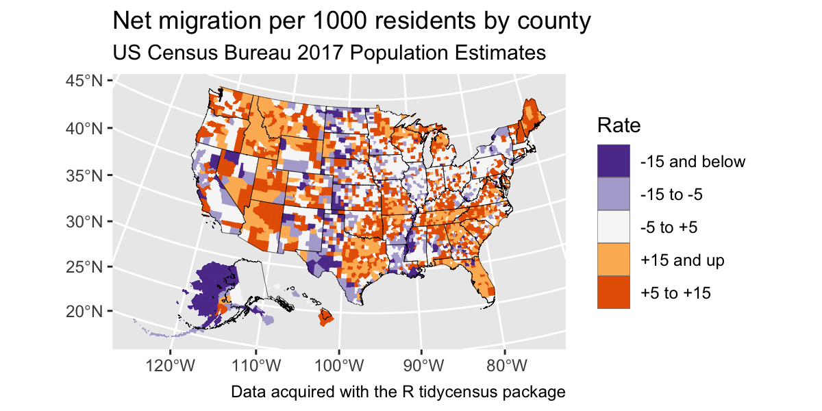
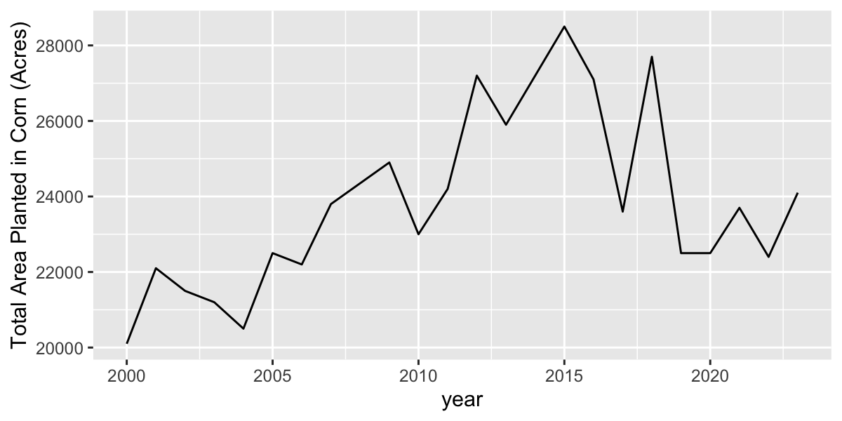
Agricultural Data
library(rnassqs)
#nassqs_auth("<your api key>")

df <- nassqs_acres(
  commodity_desc = "CORN",
  year=2000:2024,
  county_name = "Erie",
  agg_level_desc = "COUNTY",
  state_alpha = c("NY"),
  statisticcat_desc = "AREA") %>%
  filter(short_desc=="CORN - ACRES PLANTED") %>%
  dplyr::select(year, Value) %>%
  transmute(
    year = as.numeric(gsub(",", "", year)),
    value = as.numeric(gsub(",", "", Value)))
Results
geocode in ggmap package useful for geocoding place
names
Geocodes a location (find latitude and longitude) using either (1) the Data Science Toolkit (http://www.datasciencetoolkit.org/about) or (2) Google Maps.
## # A tibble: 1 × 2
##     lon   lat
##   <dbl> <dbl>
## 1 -78.8  43.0
However, you have to be careful:
## # A tibble: 1 × 2
##     lon   lat
##   <dbl> <dbl>
## 1 -77.0 38.9## # A tibble: 1 × 2
## lon lat
## <dbl> <dbl>
## 1 -77.0 38.9But this is pretty safe for well known and well-defined places.
UB=geocode("University at Buffalo, Buffalo, NY") |>
  st_as_sf(coords=c(1,2)) |> #convert to sf
  st_set_crs("+proj=longlat +ellps=WGS84 +datum=WGS84 +no_defs") |>
  st_transform(32617) |> #transform to UTM
  st_buffer(dist= 20000) |>  #radius of buffer in decimal degrees
  st_transform(4326) #transform back to longlat
Plot a leaflet map with this buffer
FedData package
- National Elevation Dataset digital elevation models (1 and 1/3 arc-second; USGS)
- National Hydrography Dataset (USGS)
- Soil Survey Geographic (SSURGO) database
- International Tree Ring Data Bank.
- Global Historical Climatology Network (GHCN)
- Others
Load FedData and define a study area
USGS National Elevation Dataset
library(rasterVis)

gplot(NED)+
  geom_raster(aes(fill=value))+
  scale_fill_viridis_c()+
  geom_sf(data=UB,inherit.aes = F,fill="transparent",col="red")+
  geom_sf(data=st_centroid(UB),inherit.aes = F,fill="transparent",col="red")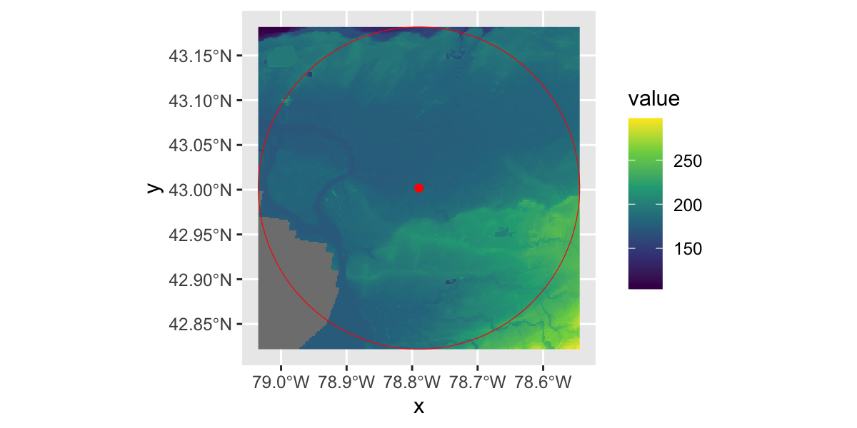
ORNL Daymet
gplot(DAYMET$tmax[[1:10]])+
  geom_raster(aes(fill=value))+
  facet_wrap(~variable)+
  scale_fill_viridis_c()+
  geom_sf(data=st_transform(UB,crs(DAYMET$tmax)),inherit.aes = F,fill="transparent",col="red")+
  labs(title="Daymet Maximum Temperature")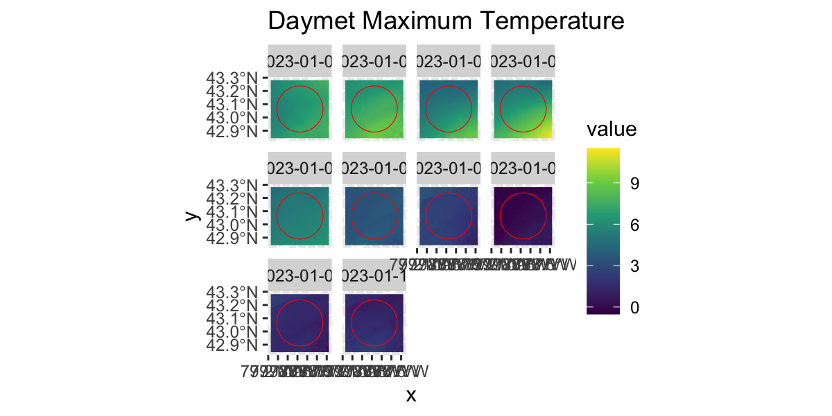
NOAA GHCN-daily
# Get the daily GHCN data (GLOBAL)
# Returns a list: the first element is the spatial locations of stations,
# and the second is a list of the stations and their daily data
GHCN.tmax <- get_ghcn_daily(
  template = UB,
  label = "UB",
  elements = c("tmax")
)

tmax <- GHCN.tmax$spatial %>%
  dplyr::mutate(label = paste0(ID, ": ", NAME))

leaflet() %>%
  addTiles() %>%
  addMarkers(data=tmax)
Reshape daily data
| STATION | YEAR | MONTH | D1 | D2 | D3 | D4 | D5 | D6 | D7 | D8 | D9 | D10 | D11 | D12 | D13 | D14 | D15 | D16 | D17 | D18 | D19 | D20 | D21 | D22 | D23 | D24 | D25 | D26 | D27 | D28 | D29 | D30 | D31 |
|---|---|---|---|---|---|---|---|---|---|---|---|---|---|---|---|---|---|---|---|---|---|---|---|---|---|---|---|---|---|---|---|---|---|
| USW00014733 | 1938 | 05 | 144 | 211 | 167 | 206 | 311 | 194 | 128 | 161 | 122 | 100 | 94 | 89 | 122 | 172 | 144 | 183 | 167 | 233 | 189 | 206 | 172 | 222 | 239 | 128 | 217 | 244 | 256 | 244 | 256 | 239 | 233 |
| USW00014733 | 1938 | 06 | 261 | 222 | 211 | 250 | 200 | 250 | 222 | 206 | 217 | 244 | 267 | 189 | 228 | 267 | 283 | 272 | 222 | 228 | 189 | 306 | 317 | 317 | 289 | 311 | 294 | 161 | 206 | 222 | 256 | 250 | NA |
| USW00014733 | 1938 | 07 | 189 | 239 | 228 | 261 | 256 | 272 | 300 | 322 | 289 | 294 | 261 | 283 | 294 | 278 | 217 | 256 | 272 | 261 | 283 | 306 | 250 | 294 | 261 | 311 | 306 | 317 | 294 | 311 | 261 | 283 | 278 |
| USW00014733 | 1938 | 08 | 256 | 289 | 322 | 300 | 311 | 289 | 317 | 306 | 300 | 267 | 267 | 250 | 267 | 294 | 306 | 317 | 283 | 272 | 306 | 311 | 300 | 283 | 261 | 228 | 211 | 239 | 256 | 250 | 278 | 189 | 283 |
| USW00014733 | 1938 | 09 | 183 | 206 | 222 | 250 | 178 | 250 | 211 | 167 | 183 | 239 | 194 | 239 | 228 | 206 | 178 | 156 | 200 | 244 | 183 | 178 | 144 | 139 | 211 | 189 | 217 | 239 | 194 | 194 | 139 | 161 | NA |
| USW00014733 | 1938 | 10 | 139 | 150 | 178 | 194 | 122 | 83 | 144 | 133 | 117 | 178 | 228 | 267 | 233 | 211 | 228 | 239 | 233 | 256 | 222 | 117 | 94 | 133 | 194 | 156 | 122 | 211 | 83 | 100 | 139 | 61 | 122 |
daily <- GHCN.tmax$tabular$USW00014733$TMAX |>
  gather(day,value,-STATION,-YEAR,-MONTH) |>
  mutate(day=str_remove(day,"D"),
         tmax=value/10,
         date=as_date(paste(YEAR,MONTH,day,sep="-"))) %>%
  arrange(date)

kable(head(daily))| STATION | YEAR | MONTH | day | value | tmax | date |
|---|---|---|---|---|---|---|
| USW00014733 | 1938 | 05 | 1 | 144 | 14.4 | 1938-05-01 |
| USW00014733 | 1938 | 05 | 2 | 211 | 21.1 | 1938-05-02 |
| USW00014733 | 1938 | 05 | 3 | 167 | 16.7 | 1938-05-03 |
| USW00014733 | 1938 | 05 | 4 | 206 | 20.6 | 1938-05-04 |
| USW00014733 | 1938 | 05 | 5 | 311 | 31.1 | 1938-05-05 |
| USW00014733 | 1938 | 05 | 6 | 194 | 19.4 | 1938-05-06 |
Plot temperatures
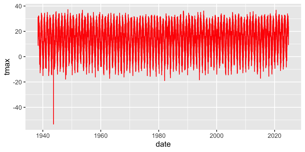
Limit to a few years
daily_recent=filter(daily,date>as.Date("2020-01-01"))

ggplot(daily_recent,
        aes(y=tmax,x=date))+
 geom_line(col="red")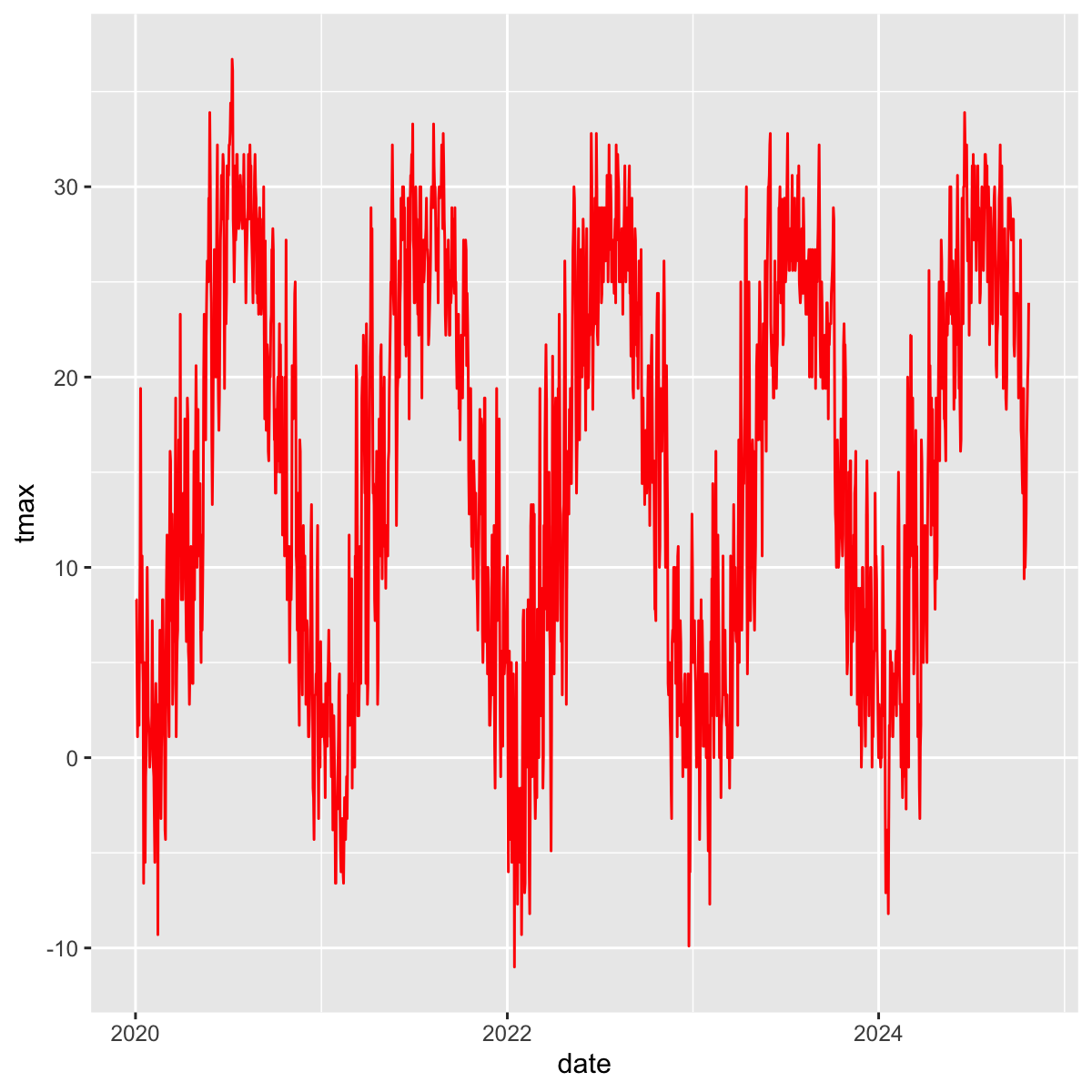
Zoo package for rolling functions
Infrastructure for Regular and Irregular Time Series (Z’s Ordered Observations)
rollmean(): Rolling meanrollsum(): Rolling sumrollapply(): Custom functions
Use rollmean to calculate a rolling 60-day average.
alignwhether the index of the result should be left- or right-aligned or centered
d_rollmean%>%
  ggplot(aes(y=tmax,x=date))+
    geom_line(col="grey")+
    geom_line(aes(y=tmax.60),col="red")+
    geom_line(aes(y=tmax.b60),col="darkred")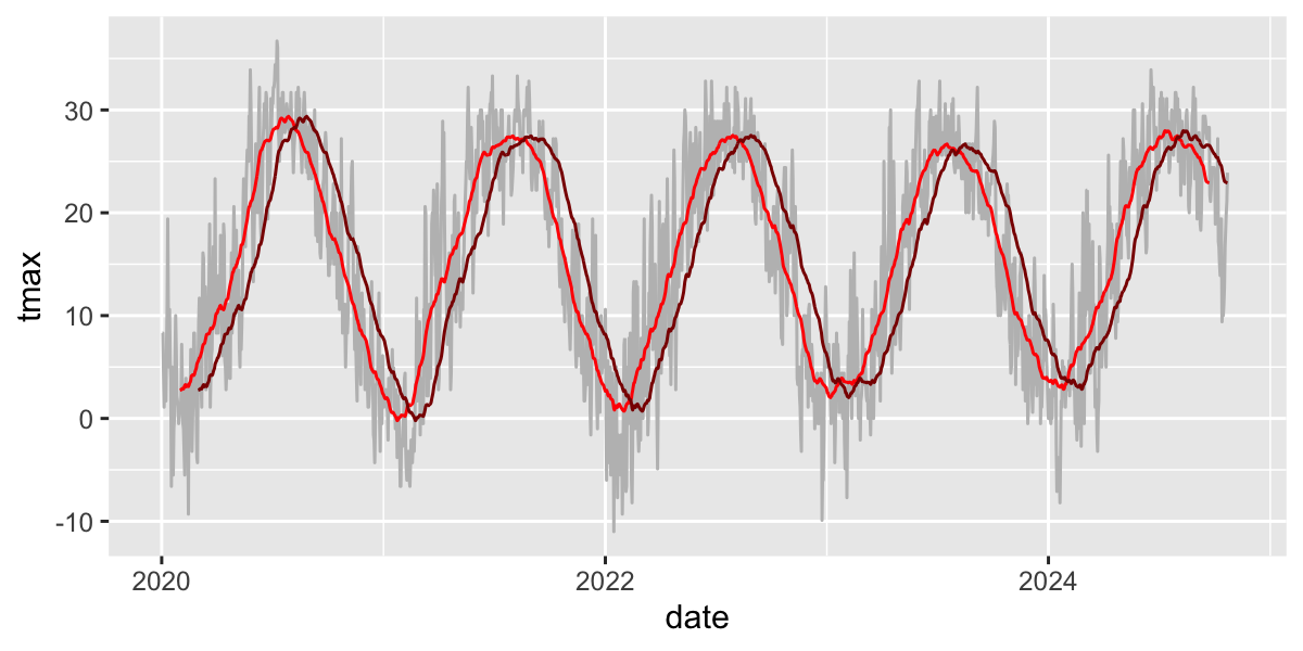
Time Series analysis
Most timeseries functions use the time series class
(ts)
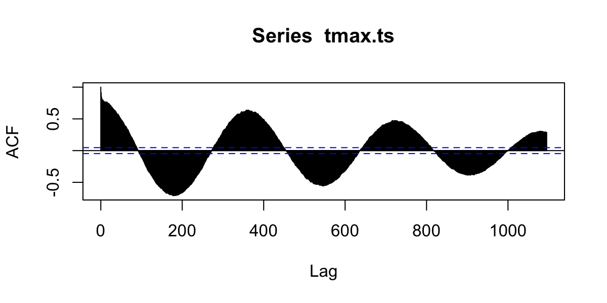
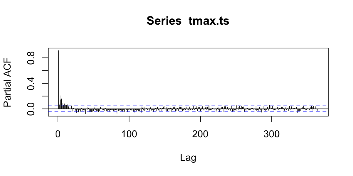
Temporal autocorrelation
Values are highly correlated!
## Warning: Removed 10 rows containing missing values or values outside the scale range
## (`geom_point()`).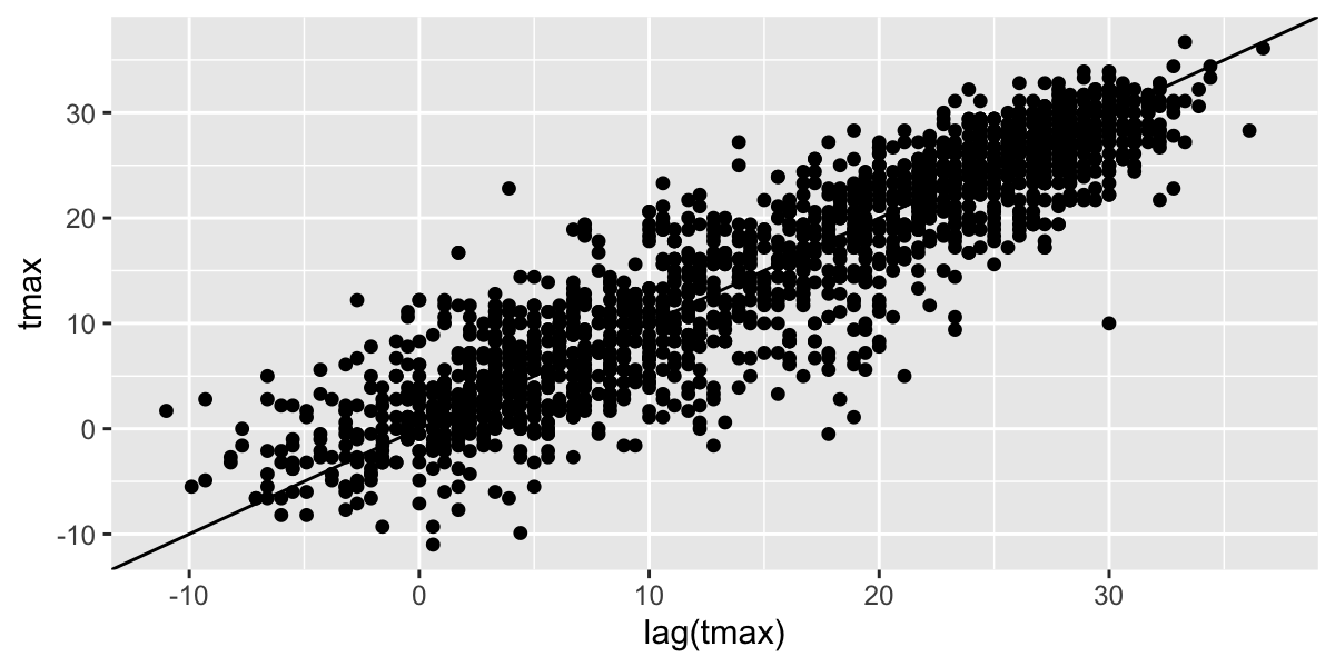
Autocorrelation functions
- autocorrelation \(x\) vs. \(x_{t-1}\) (lag=1)
- partial autocorrelation. \(x\) vs. \(x_{n}\) after controlling for correlations \(\in t-1:n\)
Autocorrelation
Partial Autocorrelation
Trend analysis
Group by month, season, year, and decade.
How to convert years into ‘decades’?
## [1] 1938## [1] 1940## [1] 193## [1] 1930Now we can make a ‘decade’ grouping variable.
Calculate seasonal and decadal mean temperatures.
daily2=daily%>%
  mutate(month=as.numeric(format(date,"%m")),
        year=as.numeric(format(date,"%Y")),
        season=case_when(
          month%in%c(12,1,2)~"Winter",
          month%in%c(3,4,5)~"Spring",
          month%in%c(6,7,8)~"Summer",
          month%in%c(9,10,11)~"Fall"),
        dec=(floor(as.numeric(format(date,"%Y"))/10)*10))
daily2%>%dplyr::select(date,month,year,season,dec,tmax)%>%head()%>%kable()| date | month | year | season | dec | tmax |
|---|---|---|---|---|---|
| 1938-05-01 | 5 | 1938 | Spring | 1930 | 14.4 |
| 1938-05-02 | 5 | 1938 | Spring | 1930 | 21.1 |
| 1938-05-03 | 5 | 1938 | Spring | 1930 | 16.7 |
| 1938-05-04 | 5 | 1938 | Spring | 1930 | 20.6 |
| 1938-05-05 | 5 | 1938 | Spring | 1930 | 31.1 |
| 1938-05-06 | 5 | 1938 | Spring | 1930 | 19.4 |
Timeseries models
How to assess change? Simple differences?
daily2%>%
  mutate(period=ifelse(year<=1976-01-01,"early","late"))%>% #create two time periods before and after 1976
  group_by(period)%>%  # divide the data into the two groups
  summarize(n=n(),    # calculate the means between the two periods
            tmax=mean(tmax,na.rm=T))%>%
kable()| period | n | tmax |
|---|---|---|
| early | 13394 | 13.65857 |
| late | 18202 | 13.89095 |
| NA | 582 | NaN |
But be careful, there were missing data in the beginning of the record
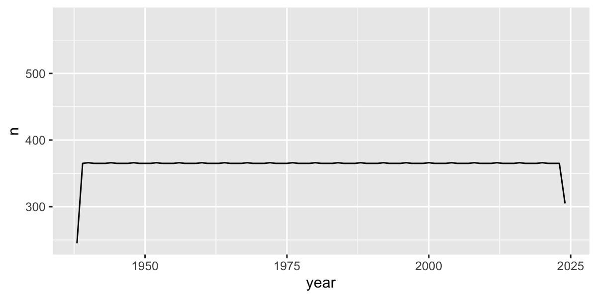
# which years don't have complete data?
daily2%>%
  group_by(year)%>%
  summarize(n=n())%>%
  filter(n<360)
## # A tibble: 2 × 2
## year n
## <dbl> <int>
## 1 1938 245
## 2 2024 305Plot 10-year means (excluding years without complete data):
daily2%>%
  filter(year>1938, year<2024)%>%
  group_by(dec)%>%
  summarize(
            n=n(),
            tmax=mean(tmax,na.rm=T)
            )%>%
  ggplot(aes(x=dec,y=tmax))+
  geom_line(col="grey")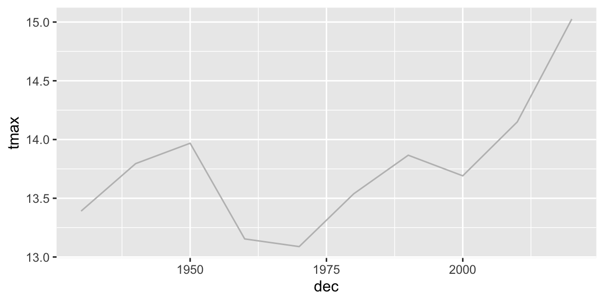
Look for specific events: was 2024 unusually hot in Buffalo, NY?
Let’s compare 2024 with all the previous years in the dataset. First add ‘day of year’ to the data to facilitate showing all years on the same plot.
Then plot all years (in grey) and add 2024 in red.
ggplot(df,aes(x=doydate,y=tmax,group=year))+
  geom_line(col="grey",alpha=.5)+ # plot each year in grey
  stat_smooth(aes(group=1),col="black")+   # Add a smooth GAM to estimate the long-term mean
  geom_line(data=filter(df,year==2024),col="red")+  # add 2023 in red
  scale_x_date(labels = date_format("%b"),date_breaks = "2 months") +
  xlab("Day of year")
## `geom_smooth()` using method = 'gam' and formula = 'y ~ s(x, bs = "cs")'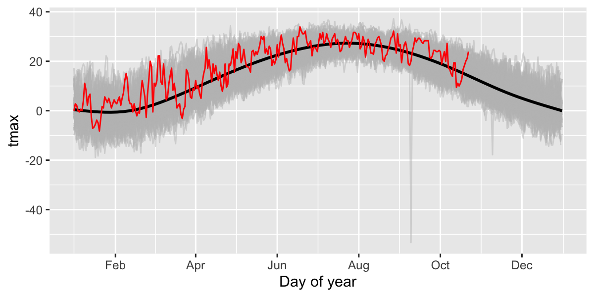
Then ‘zoom’ into just the past few months and add 2024 in red.
ggplot(df,aes(x=doydate,y=tmax,group=year))+
  geom_line(col="grey",alpha=.5)+
  stat_smooth(aes(group=1),col="black")+
  geom_line(data=filter(df,year==2024),col="red")+
  scale_x_date(labels = date_format("%b"),date_breaks = "2 months",
               lim=c(as.Date("2024-08-01"),as.Date("2024-10-31")))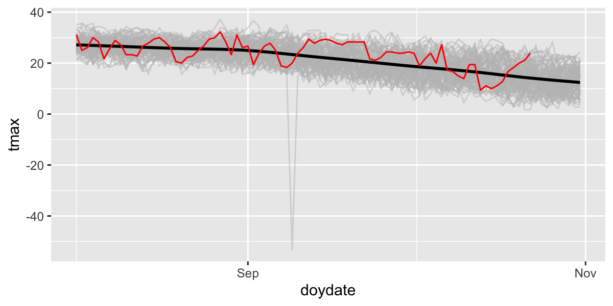
Summarize by season
Seasonal Trends
seasonal |>
    filter(!is.na(season)) |>
ggplot(aes(y=tmax,x=year))+
  facet_wrap(~season,scales = "free_y")+
  stat_smooth(method="lm", se=T)+
  geom_line()
## `geom_smooth()` using formula = 'y ~ x'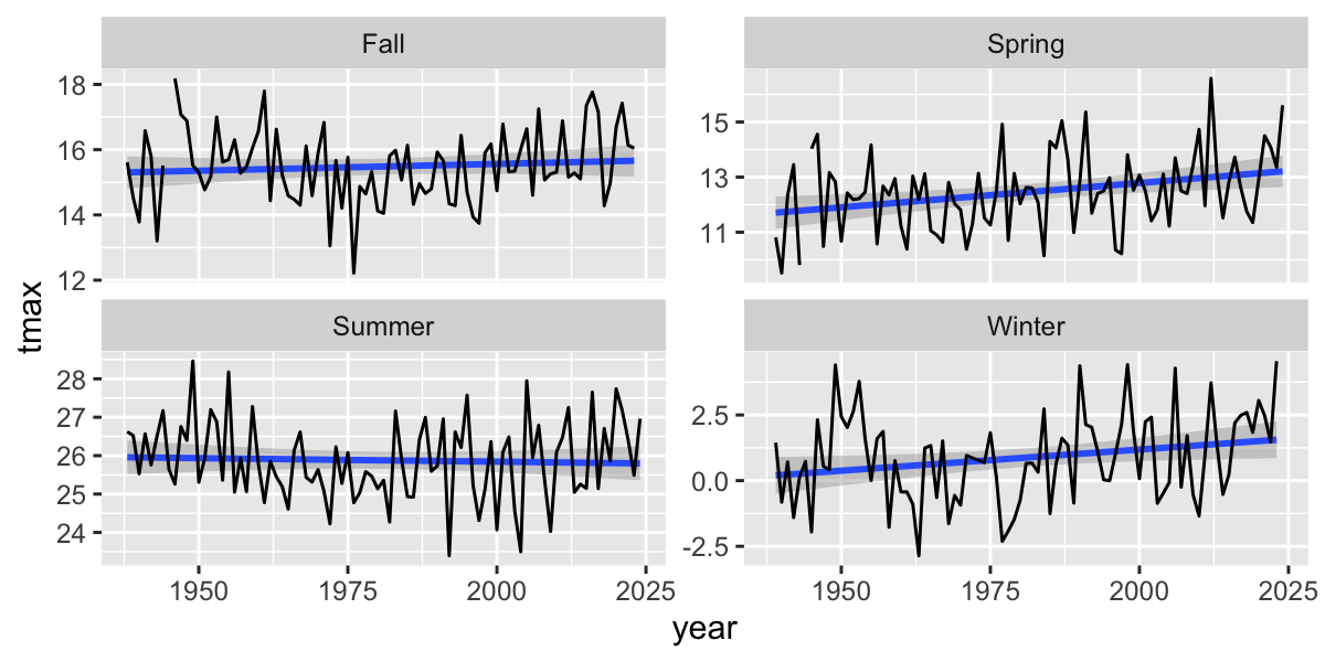
Fit a linear model to a single season
## [1] 0.002034488| term | estimate | std.error | statistic | p.value |
|---|---|---|---|---|
| (Intercept) | 29.5466595 | 8.8153619 | 3.3517240 | 0.0012002 |
| year | -0.0018523 | 0.0044496 | -0.4162739 | 0.6782588 |
Linear regression for each season
# fit a lm model for each group
  daily2 %>%
  filter(!is.na(season)) |>
  group_by(season) %>% #process by season
  nest() %>% # cut into groups
  mutate(
    lm_tmax = purrr::map(data, .f = ~ lm(tmax ~ year, data = .)), #fit model for each group
    tmax_tidy = purrr::map(lm_tmax, broom::tidy) #summarize model for each group
  ) %>%
  unnest(tmax_tidy) %>%
  filter(term == "year") %>%
  dplyr::select(-data, -lm_tmax) %>%
kable()| season | term | estimate | std.error | statistic | p.value |
|---|---|---|---|---|---|
| Spring | year | 0.0155728 | 0.0038701 | 4.023831 | 0.0000578 |
| Summer | year | -0.0018523 | 0.0017078 | -1.084612 | 0.2781264 |
| Fall | year | 0.0068981 | 0.0034962 | 1.973021 | 0.0485281 |
| Winter | year | 0.0165141 | 0.0028321 | 5.830986 | 0.0000000 |
Autoregressive models
See Time Series Analysis Task View for summary of available pack,-ages/models.
- Moving average (MA) models
- autoregressive (AR) models
- autoregressive moving average (ARMA) models
- frequency analysis
- Many, many more…