Joining / Merging Data
Today’s agenda
- Q&A
- Resource Presentation
- Case Study Presentations
- Case Study Introduction
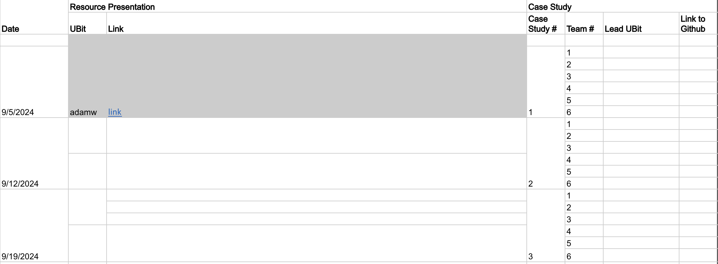
Course Schedule
Resource Presentations
Case Study Presentations - Let’s pick a winner!
Next Week’s Case Study
Data manipulation tools
dplyr and the tidyverse
Data camp tidyverse course!!
filter()mutate()summarize()group_by()
Relational Data
Flight Table inlibrary(nycflights13)
| year | month | day | dep_time | sched_dep_time | dep_delay | arr_time | sched_arr_time | arr_delay | carrier | flight | tailnum | origin | dest | air_time | distance | hour | minute | time_hour |
|---|---|---|---|---|---|---|---|---|---|---|---|---|---|---|---|---|---|---|
| 2013 | 1 | 1 | 517 | 515 | 2 | 830 | 819 | 11 | UA | 1545 | N14228 | EWR | IAH | 227 | 1400 | 5 | 15 | 2013-01-01 05:00:00 |
| 2013 | 1 | 1 | 533 | 529 | 4 | 850 | 830 | 20 | UA | 1714 | N24211 | LGA | IAH | 227 | 1416 | 5 | 29 | 2013-01-01 05:00:00 |
| 2013 | 1 | 1 | 542 | 540 | 2 | 923 | 850 | 33 | AA | 1141 | N619AA | JFK | MIA | 160 | 1089 | 5 | 40 | 2013-01-01 05:00:00 |
| 2013 | 1 | 1 | 544 | 545 | -1 | 1004 | 1022 | -18 | B6 | 725 | N804JB | JFK | BQN | 183 | 1576 | 5 | 45 | 2013-01-01 05:00:00 |
| 2013 | 1 | 1 | 554 | 600 | -6 | 812 | 837 | -25 | DL | 461 | N668DN | LGA | ATL | 116 | 762 | 6 | 0 | 2013-01-01 06:00:00 |
| 2013 | 1 | 1 | 554 | 558 | -4 | 740 | 728 | 12 | UA | 1696 | N39463 | EWR | ORD | 150 | 719 | 5 | 58 | 2013-01-01 05:00:00 |
| 2013 | 1 | 1 | 555 | 600 | -5 | 913 | 854 | 19 | B6 | 507 | N516JB | EWR | FLL | 158 | 1065 | 6 | 0 | 2013-01-01 06:00:00 |
| 2013 | 1 | 1 | 557 | 600 | -3 | 709 | 723 | -14 | EV | 5708 | N829AS | LGA | IAD | 53 | 229 | 6 | 0 | 2013-01-01 06:00:00 |
| 2013 | 1 | 1 | 557 | 600 | -3 | 838 | 846 | -8 | B6 | 79 | N593JB | JFK | MCO | 140 | 944 | 6 | 0 | 2013-01-01 06:00:00 |
| 2013 | 1 | 1 | 558 | 600 | -2 | 753 | 745 | 8 | AA | 301 | N3ALAA | LGA | ORD | 138 | 733 | 6 | 0 | 2013-01-01 06:00:00 |
Airport table in
library(nycflights13)
| faa | name | lat | lon | alt | tz | dst | tzone |
|---|---|---|---|---|---|---|---|
| 04G | Lansdowne Airport | 41.13047 | -80.61958 | 1044 | -5 | A | America/New_York |
| 06A | Moton Field Municipal Airport | 32.46057 | -85.68003 | 264 | -6 | A | America/Chicago |
| 06C | Schaumburg Regional | 41.98934 | -88.10124 | 801 | -6 | A | America/Chicago |
| 06N | Randall Airport | 41.43191 | -74.39156 | 523 | -5 | A | America/New_York |
| 09J | Jekyll Island Airport | 31.07447 | -81.42778 | 11 | -5 | A | America/New_York |
| 0A9 | Elizabethton Municipal Airport | 36.37122 | -82.17342 | 1593 | -5 | A | America/New_York |
| 0G6 | Williams County Airport | 41.46731 | -84.50678 | 730 | -5 | A | America/New_York |
| 0G7 | Finger Lakes Regional Airport | 42.88356 | -76.78123 | 492 | -5 | A | America/New_York |
| 0P2 | Shoestring Aviation Airfield | 39.79482 | -76.64719 | 1000 | -5 | U | America/New_York |
| 0S9 | Jefferson County Intl | 48.05381 | -122.81064 | 108 | -8 | A | America/Los_Angeles |
Relational Data
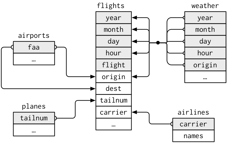
Visualizing Relational Data
- Primary key: uniquely identifies an observation in
its own table. For example,
planes$tailnumis a primary key because it uniquely identifies each plane in the planes table. - Foreign key: uniquely identifies an observation in
another table. For example, the
flights$tailnumis a foreign key because it appears in the flights table where it matches each flight to a unique plane.
3 families of verbs designed to work with relational data
- Mutating joins: add new variables to one data frame from matching observations in another
- Filtering joins: filter observations from one data frame based on whether or not they match an observation in the other table.
- Set operations: treat observations as if they were set elements
Inner Join
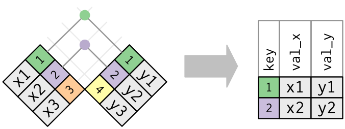
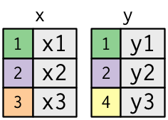
Matches pairs of observations whenever their keys are equal:
Outer Joins
left_joinkeeps all observations in xright_joinkeeps all observations in yfull_joinkeeps all observations in x and y
Outer Joins
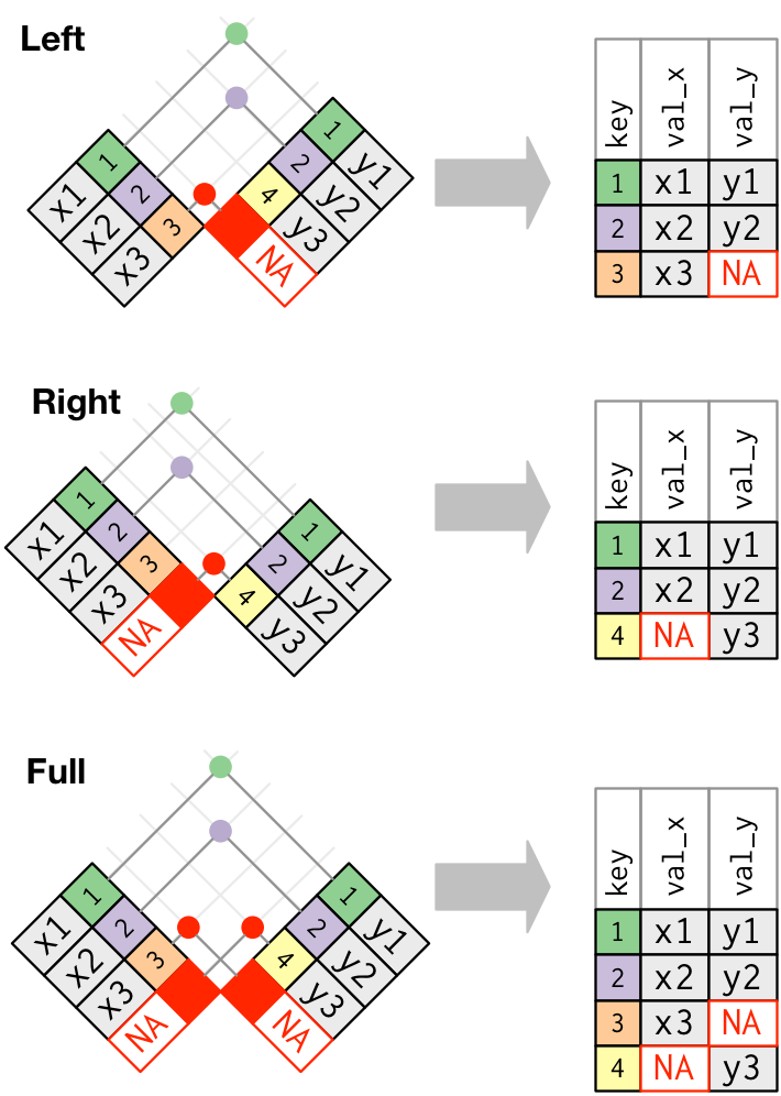
Outer Joins: another visualization

Potential Problems
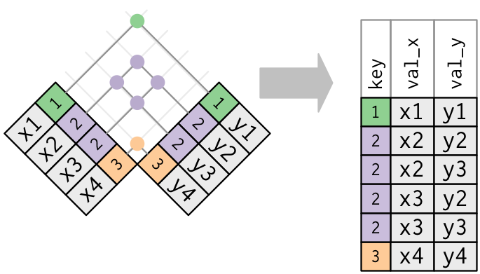
Duplicate Keys
One table w/ duplicates
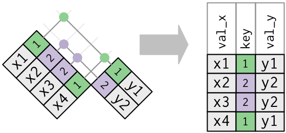
Duplicate Keys
Both tables w/ duplicates
Missing Keys
semi_join(x, y)
keeps all observations in x that have a match in y.
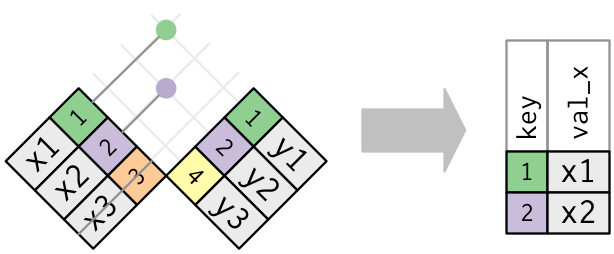
anti_join(x, y) drops all observations in x that have a
match in y.
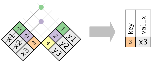
Anti-joins are useful for diagnosing join mismatches.
Compare with other functions
merge()
base::merge() can perform all four types of joins:
| dplyr | merge |
|---|---|
inner_join(x, y) |
merge(x, y) |
left_join(x, y) |
merge(x, y, all.x = TRUE) |
right_join(x, y) |
merge(x, y, all.y = TRUE) |
full_join(x, y) |
merge(x, y, all.x = TRUE, all.y = TRUE) |
- specific dplyr verbs more clearly convey the intent of your code: they are concealed in the arguments of merge().
- dplyr’s joins are considerably faster and don’t mess with the order of the rows.
SQL
SQL is the inspiration for dplyr’s conventions, so the translation is straightforward:
| dplyr | SQL |
|---|---|
inner_join(x, y, by = "z") |
SELECT * FROM x INNER JOIN y USING (z) |
left_join(x, y, by = "z") |
SELECT * FROM x LEFT OUTER JOIN y USING (z) |
right_join(x, y, by = "z") |
SELECT * FROM x RIGHT OUTER JOIN y USING (z) |
full_join(x, y, by = "z") |
SELECT * FROM x FULL OUTER JOIN y USING (z) |
- Note that “INNER” and “OUTER” are optional, and often omitted.
- SQL supports a wider range of join types than dplyr
Set Operations
intersect(x, y): return only observations in both x and y.union(x, y): return unique observations in x and y.setdiff(x, y): return observations in x, but not in y.
