Tasks

Extract a timeseries from a single location in a netcdf file (part 1)
Calculate a monthly climatology from a weekely timeseries (part 2)
Summarize Land Surface Temperature by Land Cover (part 3)

The R Script associated with this page is available here. If you like, you can download this file and open it (or copy-paste into a new script) with RStudio so you can follow along.

Libraries

library(raster)
library(rasterVis)
library(ggmap)
library(tidyverse)
library(knitr)

# New Packages
library(ncdf4) # to import data from netcdf format

Case Study Set up

Identify (and create) download folders

Today we’ll work with:

Land Surface Temperature (lst): MOD11A2
Land Cover (lc): MCD12Q1

Land Use Land Cover

# Create afolder to hold the downloaded data
dir.create("data",showWarnings = F) #create a folder to hold the data

lulc_url="https://github.com/adammwilson/DataScienceData/blob/master/inst/extdata/appeears/MCD12Q1.051_aid0001.nc?raw=true"
lst_url="https://github.com/adammwilson/DataScienceData/blob/master/inst/extdata/appeears/MOD11A2.006_aid0001.nc?raw=true"

# download them
download.file(lulc_url,destfile="data/MCD12Q1.051_aid0001.nc", mode="wb")
download.file(lst_url,destfile="data/MOD11A2.006_aid0001.nc", mode="wb")

You should also edit your .gitignore file (in your tasks repository folder) to include *data* on one line. This will prevent git from adding these files.

Load data into R

lulc=stack("data/MCD12Q1.051_aid0001.nc",varname="Land_Cover_Type_1")
lst=stack("data/MOD11A2.006_aid0001.nc",varname="LST_Day_1km")

You will probably see some errors about

>>>> WARNING <<<  attribute longitude_of_projection_origin is an 8-byte value, but R"
[1] "does not support this data type. I am returning a double precision"
[1] "floating point, but you must be aware that this could lose precision!"

You can safely ignore this.

Explore LULC data

plot(lulc)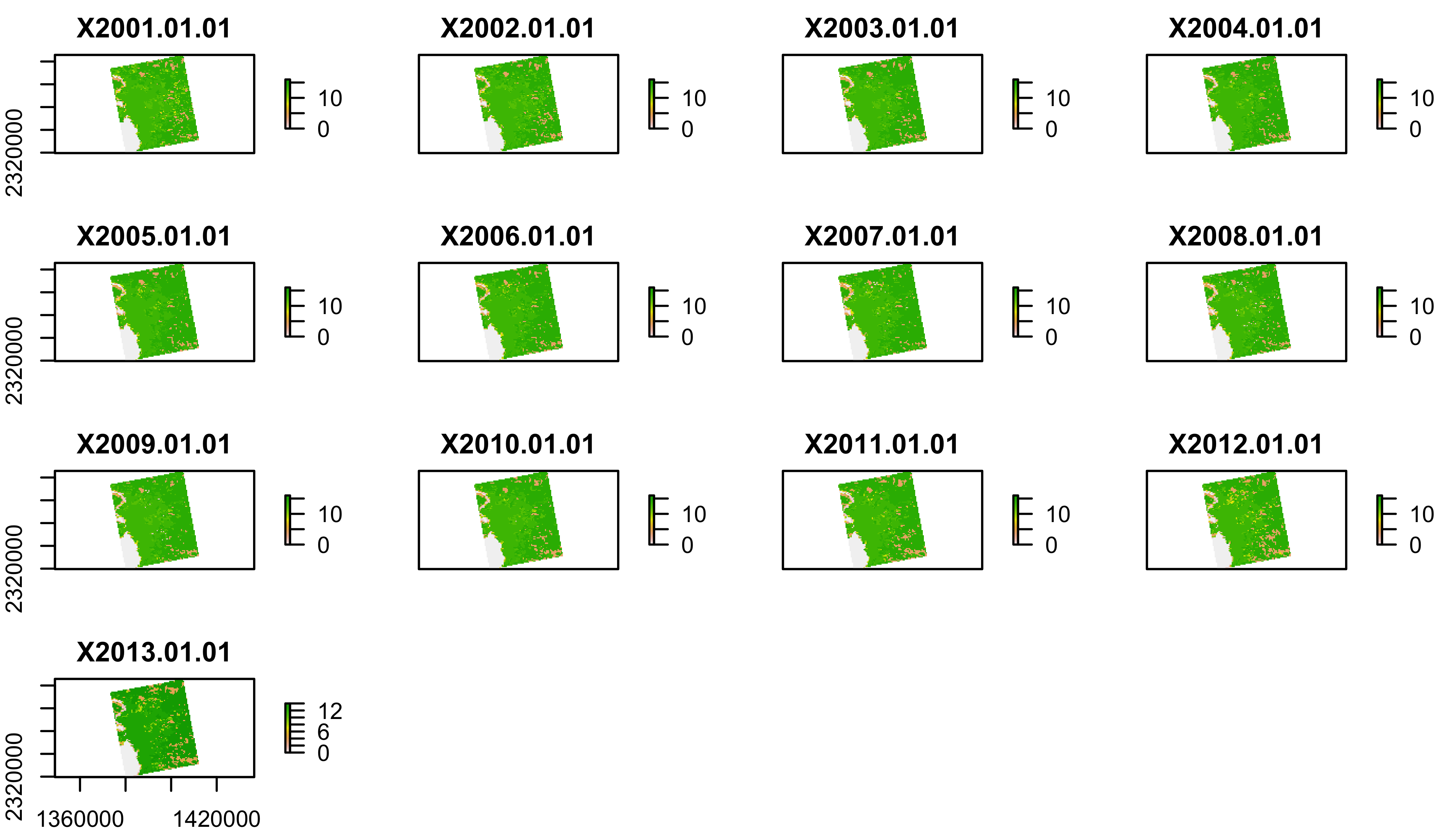

We’ll just pick one year to work with to keep this simple:

lulc=lulc[[13]]
plot(lulc)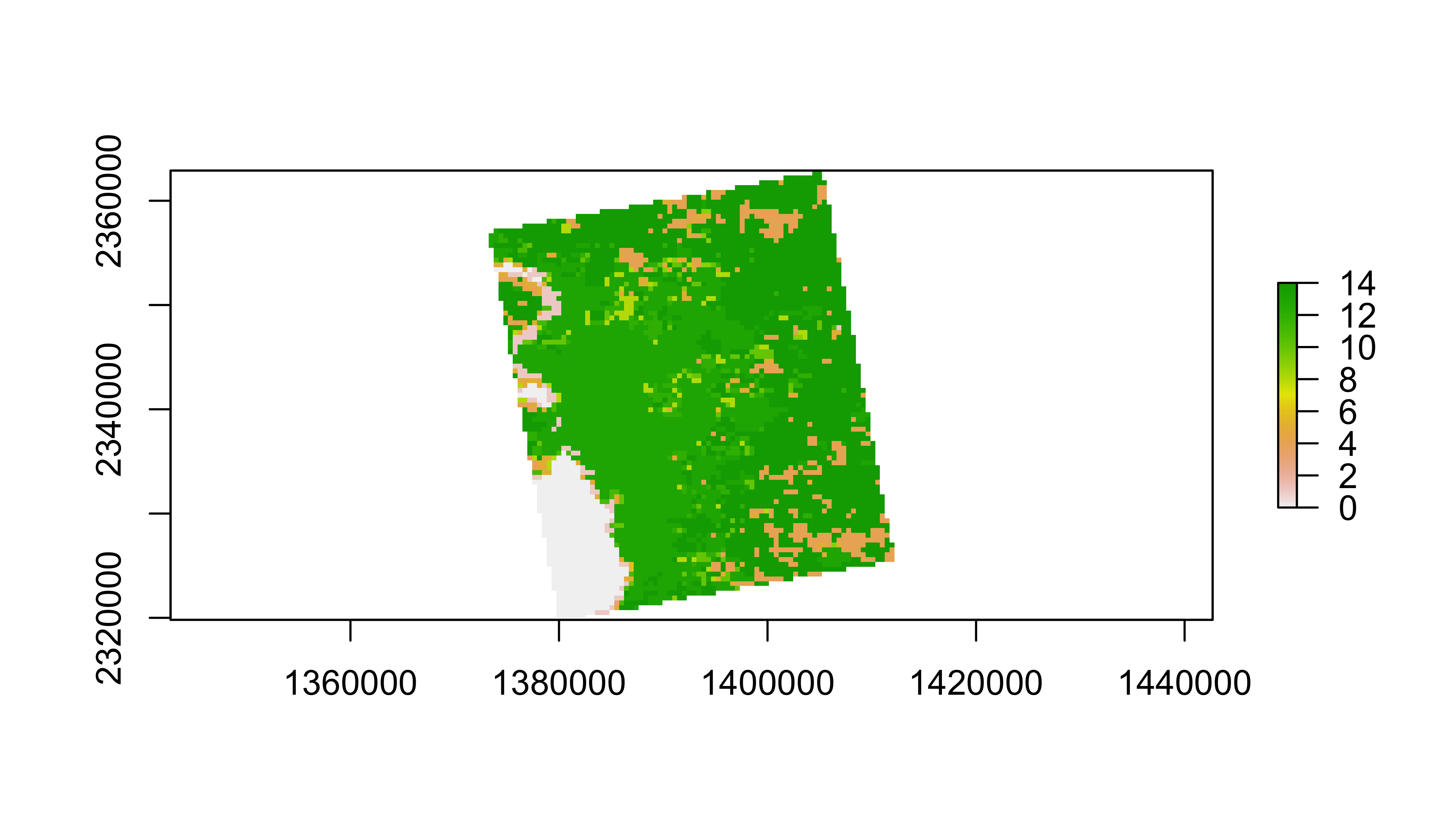

Process landcover data

Assign land cover clases from MODIS website

  Land_Cover_Type_1 = c(
    Water = 0, 
    `Evergreen Needleleaf forest` = 1, 
    `Evergreen Broadleaf forest` = 2,
    `Deciduous Needleleaf forest` = 3, 
    `Deciduous Broadleaf forest` = 4,
    `Mixed forest` = 5, 
    `Closed shrublands` = 6,
    `Open shrublands` = 7,
    `Woody savannas` = 8, 
    Savannas = 9,
    Grasslands = 10,
    `Permanent wetlands` = 11, 
    Croplands = 12,
    `Urban & built-up` = 13,
    `Cropland/Natural vegetation mosaic` = 14, 
    `Snow & ice` = 15,
    `Barren/Sparsely vegetated` = 16, 
    Unclassified = 254,
    NoDataFill = 255)

lcd=data.frame(
  ID=Land_Cover_Type_1,
  landcover=names(Land_Cover_Type_1),
  col=c("#000080","#008000","#00FF00", "#99CC00","#99FF99", "#339966", "#993366", "#FFCC99", "#CCFFCC", "#FFCC00", "#FF9900", "#006699", "#FFFF00", "#FF0000", "#999966", "#FFFFFF", "#808080", "#000000", "#000000"),
  stringsAsFactors = F)
# colors from https://lpdaac.usgs.gov/about/news_archive/modisterra_land_cover_types_yearly_l3_global_005deg_cmg_mod12c1
kable(head(lcd))

	ID	landcover	col
Water	0	Water	#000080
Evergreen Needleleaf forest	1	Evergreen Needleleaf forest	#008000
Evergreen Broadleaf forest	2	Evergreen Broadleaf forest	#00FF00
Deciduous Needleleaf forest	3	Deciduous Needleleaf forest	#99CC00
Deciduous Broadleaf forest	4	Deciduous Broadleaf forest	#99FF99
Mixed forest	5	Mixed forest	#339966

Convert LULC raster into a ‘factor’ (categorical) raster. This requires building the Raster Attribute Table (RAT). Unfortunately, this is a bit of manual process as follows.

# convert to raster (easy)
lulc=as.factor(lulc)

# update the RAT with a left join
levels(lulc)=left_join(levels(lulc)[[1]],lcd)

## Joining with `by = join_by(ID)`

# plot it
gplot(lulc)+
  geom_raster(aes(fill=as.factor(value)))+
  scale_fill_manual(values=levels(lulc)[[1]]$col,
                    labels=levels(lulc)[[1]]$landcover,
                    name="Landcover Type")+
  coord_equal()+
  theme(legend.position = "bottom")+
  guides(fill=guide_legend(ncol=1,byrow=TRUE))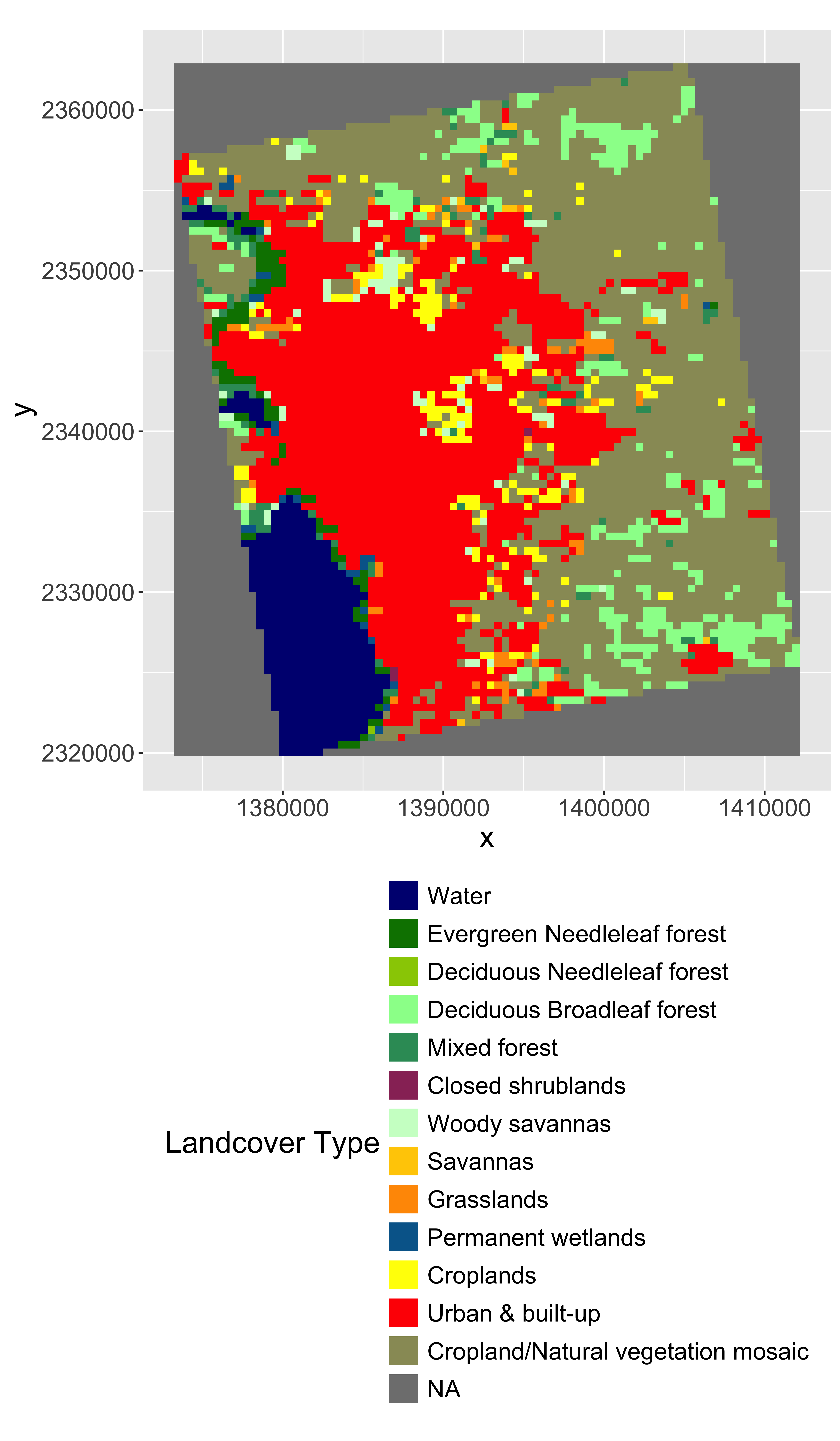

Land Surface Temperature

plot(lst[[1:12]])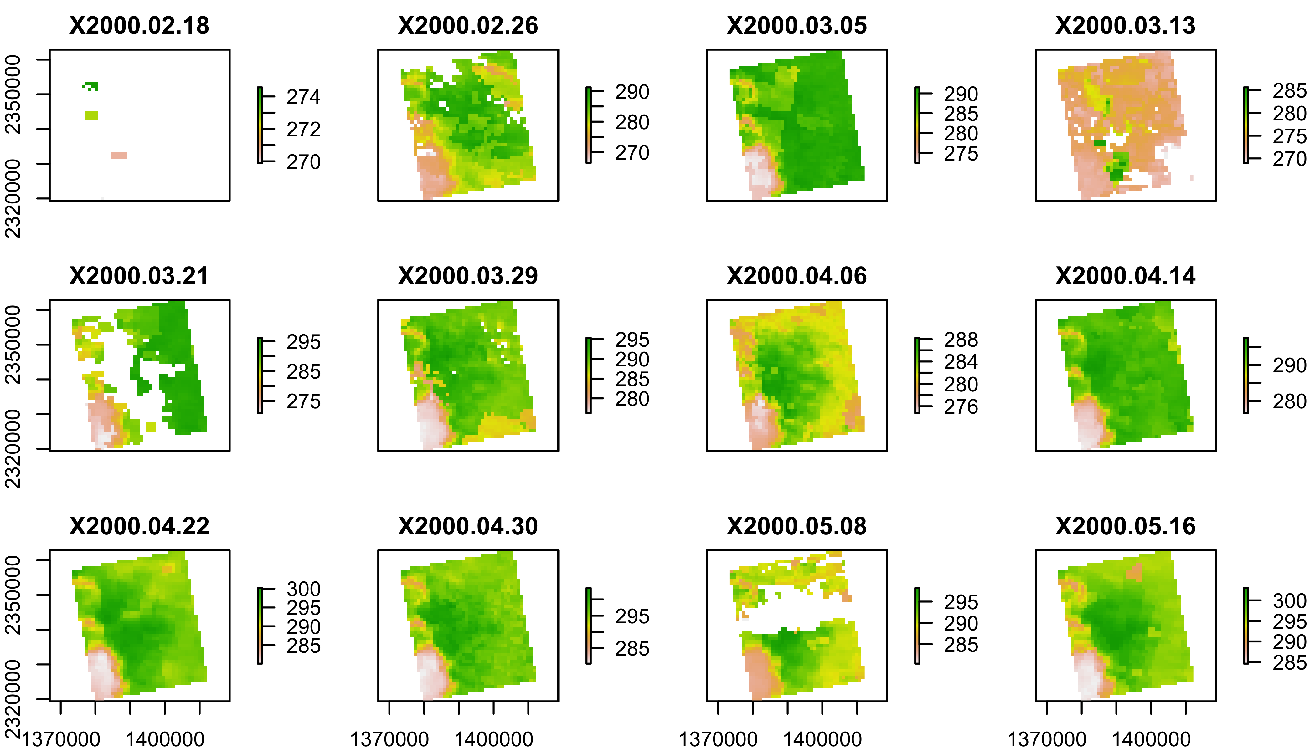

Convert LST to Degrees C

You can convert LST from Degrees Kelvin (K) to Celcius (C) with offs().

offs(lst)=-273.15
plot(lst[[1:10]])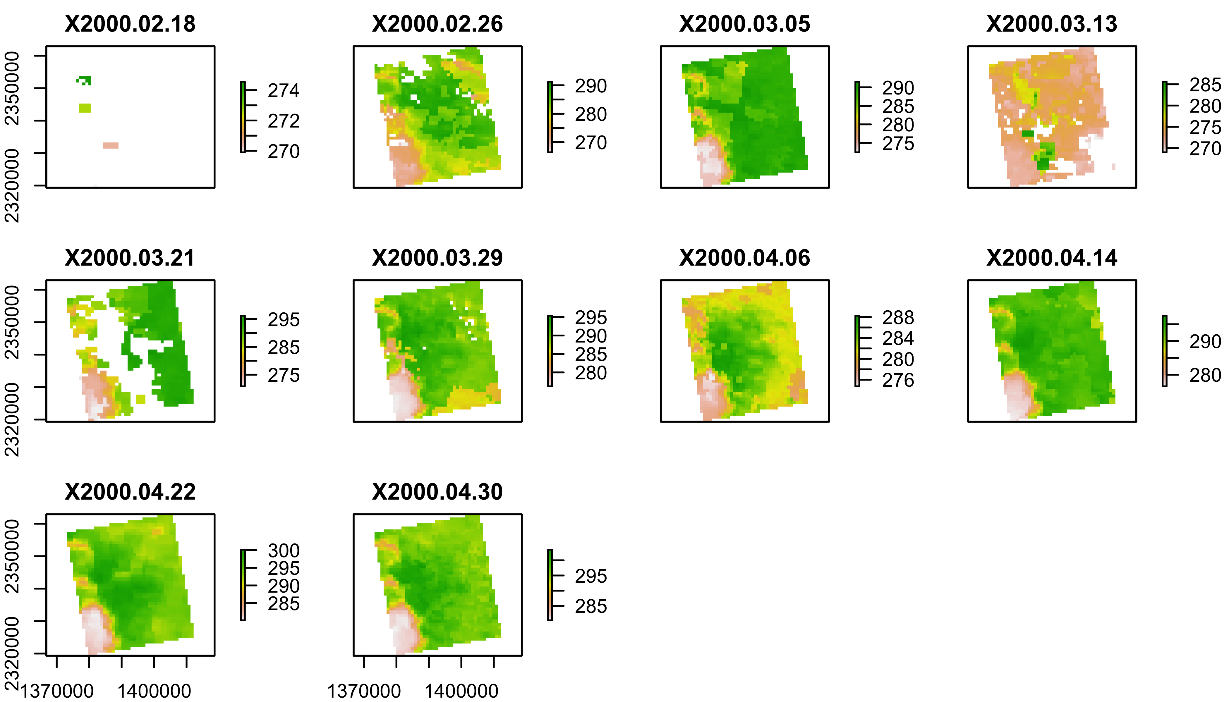

MODLAND Quality control

See a detailed explaination here. Some code below from Steven Mosher’s blog.

Expand this to learn more about MODIS quality control. This is optional for this class, but important if you want to work with this kind of data ‘for real’.

MOD11A2 (Land Surface Temperature) Quality Control

MOD11A2 QC Layer table

lstqc=stack("data/MOD11A2.006_aid0001.nc",varname="QC_Day")
plot(lstqc[[1:2]])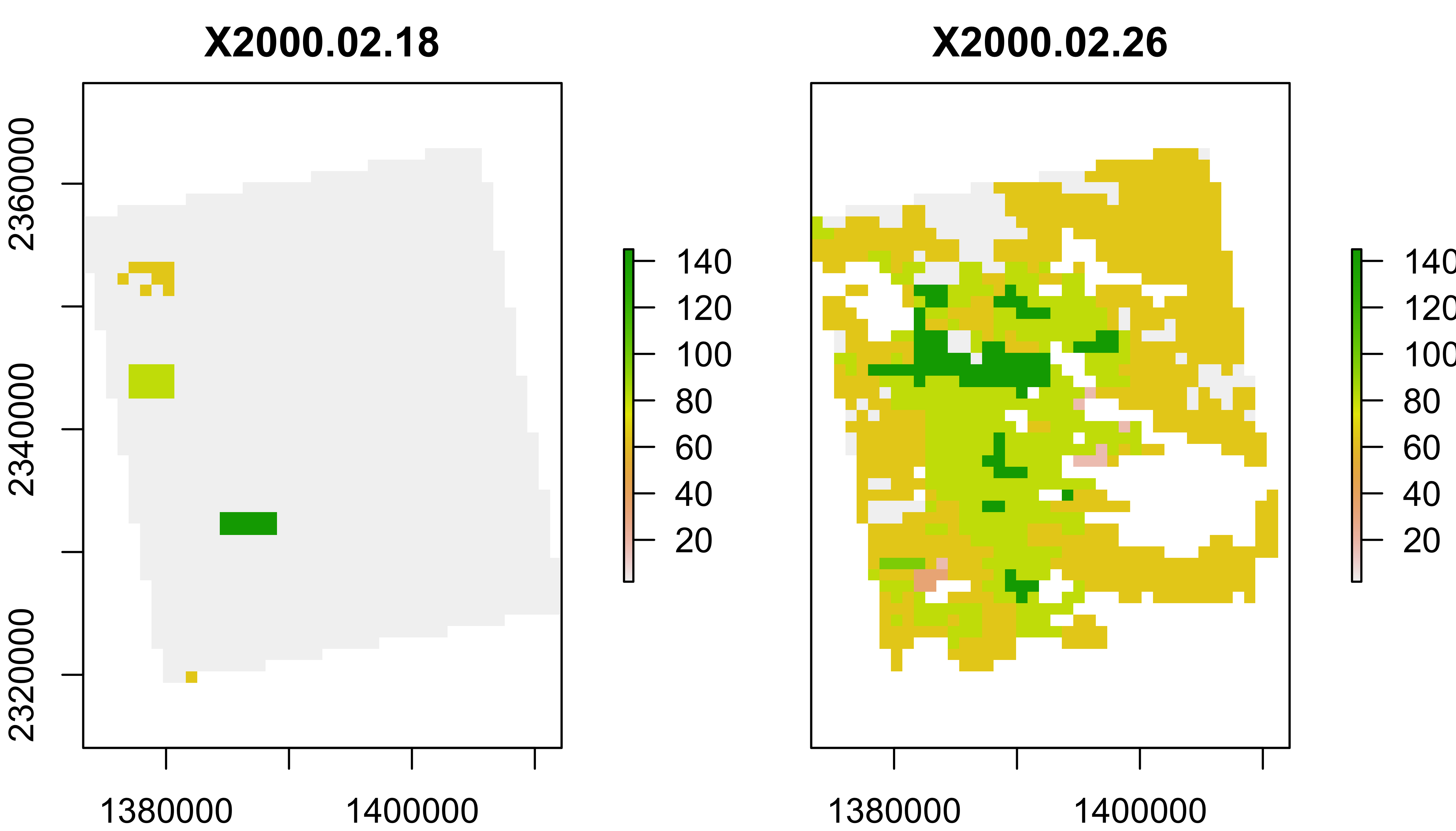

LST QC data

QC data are encoded in 8-bit ‘words’ to compress information.

values(lstqc[[1:2]])%>%table()

## .
##    2   17   33   65   81   97  145 
## 1569    8    5  675  335    4   90

intToBits(65)

##  [1] 01 00 00 00 00 00 01 00 00 00 00 00 00 00 00 00 00 00 00 00 00 00 00 00 00
## [26] 00 00 00 00 00 00 00

intToBits(65)[1:8]

## [1] 01 00 00 00 00 00 01 00

as.integer(intToBits(65)[1:8])

## [1] 1 0 0 0 0 0 1 0

MODIS QC data are Big Endian

Format	Digits	value	sum
Little Endian	1 0 0 0 0 0 1 0	65	2^0 + 2^6
Big Endian	0 1 0 0 0 0 0 1	65	2^6 + 2^0

Reverse the digits with rev() and compare with QC table above.

rev(as.integer(intToBits(65)[1:8]))

## [1] 0 1 0 0 0 0 0 1

QC for value 65:

LST produced, other quality, recommend examination of more detailed QA
good data quality of L1B in 7 TIR bands
average emissivity error <= 0.01
Average LST error <= 2K

Filter the the lst data using the QC data

## set up data frame to hold all combinations
QC_Data <- data.frame(Integer_Value = 0:255,
Bit7 = NA, Bit6 = NA, Bit5 = NA, Bit4 = NA,
Bit3 = NA, Bit2 = NA, Bit1 = NA, Bit0 = NA,
QA_word1 = NA, QA_word2 = NA, QA_word3 = NA,
QA_word4 = NA)

## 
for(i in QC_Data$Integer_Value){
AsInt <- as.integer(intToBits(i)[1:8])
QC_Data[i+1,2:9]<- AsInt[8:1]
}

QC_Data$QA_word1[QC_Data$Bit1 == 0 & QC_Data$Bit0==0] <- "LST GOOD"
QC_Data$QA_word1[QC_Data$Bit1 == 0 & QC_Data$Bit0==1] <- "LST Produced,Other Quality"
QC_Data$QA_word1[QC_Data$Bit1 == 1 & QC_Data$Bit0==0] <- "No Pixel,clouds"
QC_Data$QA_word1[QC_Data$Bit1 == 1 & QC_Data$Bit0==1] <- "No Pixel, Other QA"

QC_Data$QA_word2[QC_Data$Bit3 == 0 & QC_Data$Bit2==0] <- "Good Data"
QC_Data$QA_word2[QC_Data$Bit3 == 0 & QC_Data$Bit2==1] <- "Other Quality"
QC_Data$QA_word2[QC_Data$Bit3 == 1 & QC_Data$Bit2==0] <- "TBD"
QC_Data$QA_word2[QC_Data$Bit3 == 1 & QC_Data$Bit2==1] <- "TBD"

QC_Data$QA_word3[QC_Data$Bit5 == 0 & QC_Data$Bit4==0] <- "Emiss Error <= .01"
QC_Data$QA_word3[QC_Data$Bit5 == 0 & QC_Data$Bit4==1] <- "Emiss Err >.01 <=.02"
QC_Data$QA_word3[QC_Data$Bit5 == 1 & QC_Data$Bit4==0] <- "Emiss Err >.02 <=.04"
QC_Data$QA_word3[QC_Data$Bit5 == 1 & QC_Data$Bit4==1] <- "Emiss Err > .04"

QC_Data$QA_word4[QC_Data$Bit7 == 0 & QC_Data$Bit6==0] <- "LST Err <= 1"
QC_Data$QA_word4[QC_Data$Bit7 == 0 & QC_Data$Bit6==1] <- "LST Err > 2 LST Err <= 3"
QC_Data$QA_word4[QC_Data$Bit7 == 1 & QC_Data$Bit6==0] <- "LST Err > 1 LST Err <= 2"
QC_Data$QA_word4[QC_Data$Bit7 == 1 & QC_Data$Bit6==1] <- "LST Err > 4"
kable(head(QC_Data))

Integer_Value	Bit2	Bit1	Bit0	QA_word1	QA_word2	QA_word3	QA_word4
0	0	0	0	LST GOOD	Good Data	Emiss Error <= .01	LST Err <= 1
1	0	0	1	LST Produced,Other Quality	Good Data	Emiss Error <= .01	LST Err <= 1
2	0	1	0	No Pixel,clouds	Good Data	Emiss Error <= .01	LST Err <= 1
3	0	1	1	No Pixel, Other QA	Good Data	Emiss Error <= .01	LST Err <= 1
4	1	0	0	LST GOOD	Other Quality	Emiss Error <= .01	LST Err <= 1
5	1	0	1	LST Produced,Other Quality	Other Quality	Emiss Error <= .01	LST Err <= 1

Select which QC Levels to keep

keep=QC_Data[QC_Data$Bit1 == 0,]
keepvals=unique(keep$Integer_Value)
keepvals

##   [1]   0   1   4   5   8   9  12  13  16  17  20  21  24  25  28  29  32  33
##  [19]  36  37  40  41  44  45  48  49  52  53  56  57  60  61  64  65  68  69
##  [37]  72  73  76  77  80  81  84  85  88  89  92  93  96  97 100 101 104 105
##  [55] 108 109 112 113 116 117 120 121 124 125 128 129 132 133 136 137 140 141
##  [73] 144 145 148 149 152 153 156 157 160 161 164 165 168 169 172 173 176 177
##  [91] 180 181 184 185 188 189 192 193 196 197 200 201 204 205 208 209 212 213
## [109] 216 217 220 221 224 225 228 229 232 233 236 237 240 241 244 245 248 249
## [127] 252 253

How many observations will be dropped?

qcvals=table(values(lstqc))  # this takes a minute or two


QC_Data%>%
  dplyr::select(everything(),-contains("Bit"))%>%
  mutate(Var1=as.character(Integer_Value),
         keep=Integer_Value%in%keepvals)%>%
  inner_join(data.frame(qcvals))%>%
  kable()

## Joining with `by = join_by(Var1)`

Integer_Value	QA_word1	QA_word2	QA_word3	QA_word4	Var1	keep	Freq
2	No Pixel,clouds	Good Data	Emiss Error <= .01	LST Err <= 1	2	FALSE	150019
17	LST Produced,Other Quality	Good Data	Emiss Err >.01 <=.02	LST Err <= 1	17	TRUE	44552
33	LST Produced,Other Quality	Good Data	Emiss Err >.02 <=.04	LST Err <= 1	33	TRUE	20225
49	LST Produced,Other Quality	Good Data	Emiss Err > .04	LST Err <= 1	49	TRUE	3
65	LST Produced,Other Quality	Good Data	Emiss Error <= .01	LST Err > 2 LST Err <= 3	65	TRUE	243391
81	LST Produced,Other Quality	Good Data	Emiss Err >.01 <=.02	LST Err > 2 LST Err <= 3	81	TRUE	203501
97	LST Produced,Other Quality	Good Data	Emiss Err >.02 <=.04	LST Err > 2 LST Err <= 3	97	TRUE	25897
113	LST Produced,Other Quality	Good Data	Emiss Err > .04	LST Err > 2 LST Err <= 3	113	TRUE	32
129	LST Produced,Other Quality	Good Data	Emiss Error <= .01	LST Err > 1 LST Err <= 2	129	TRUE	57
145	LST Produced,Other Quality	Good Data	Emiss Err >.01 <=.02	LST Err > 1 LST Err <= 2	145	TRUE	29607
161	LST Produced,Other Quality	Good Data	Emiss Err >.02 <=.04	LST Err > 1 LST Err <= 2	161	TRUE	3
177	LST Produced,Other Quality	Good Data	Emiss Err > .04	LST Err > 1 LST Err <= 2	177	TRUE	5

Do you want to update the values you are keeping?

Filter the LST Data keeping only `keepvals`

These steps take a couple minutes.

Make logical flag to use for mask

lstkeep=calc(lstqc,function(x) x%in%keepvals)

Plot the mask

gplot(lstkeep[[4:8]])+
  geom_raster(aes(fill=as.factor(value)))+
  facet_grid(variable~.)+
  scale_fill_manual(values=c("blue","red"),name="Keep")+
  coord_equal()+
  theme(legend.position = "bottom")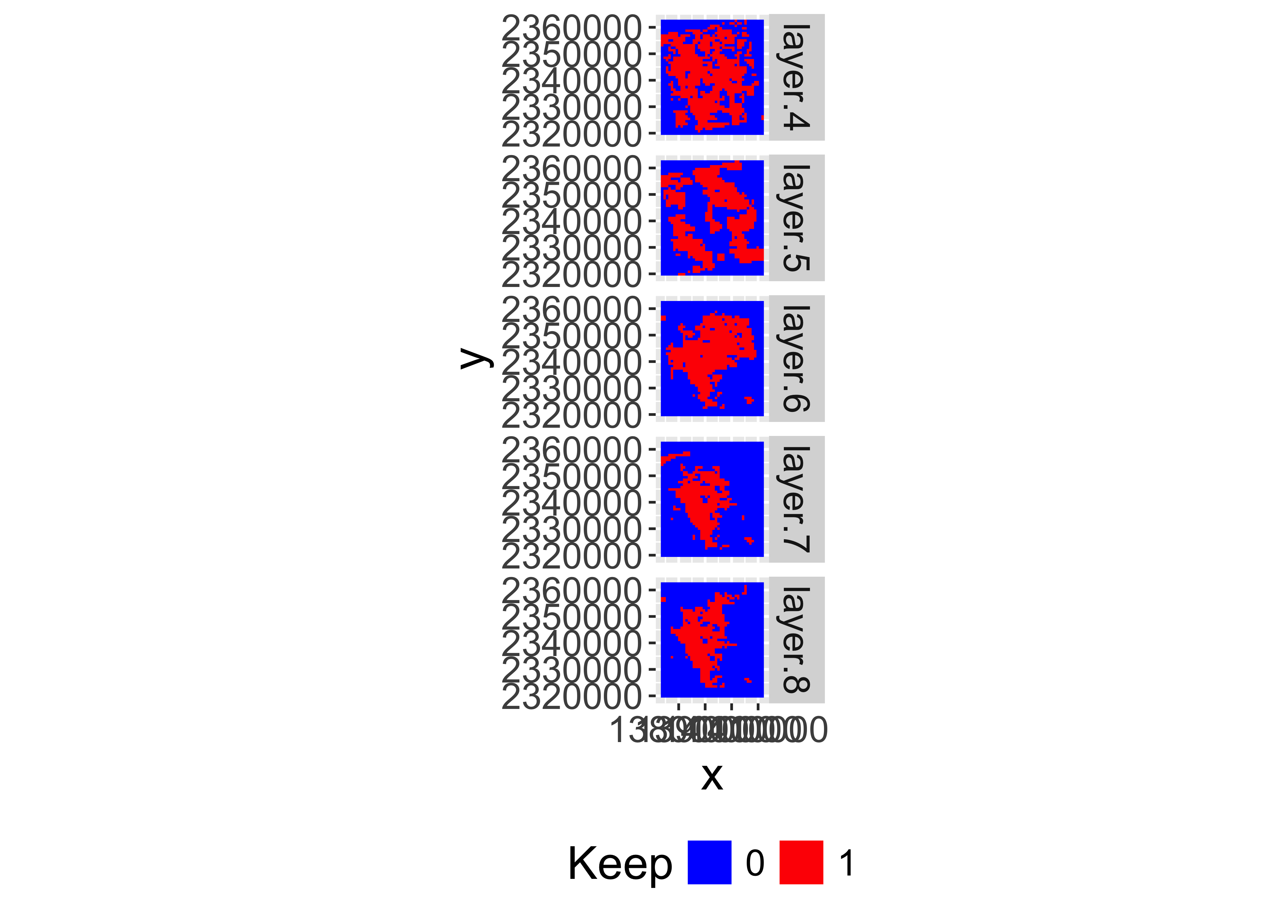

Mask the lst data using the QC data and overwrite the original data.

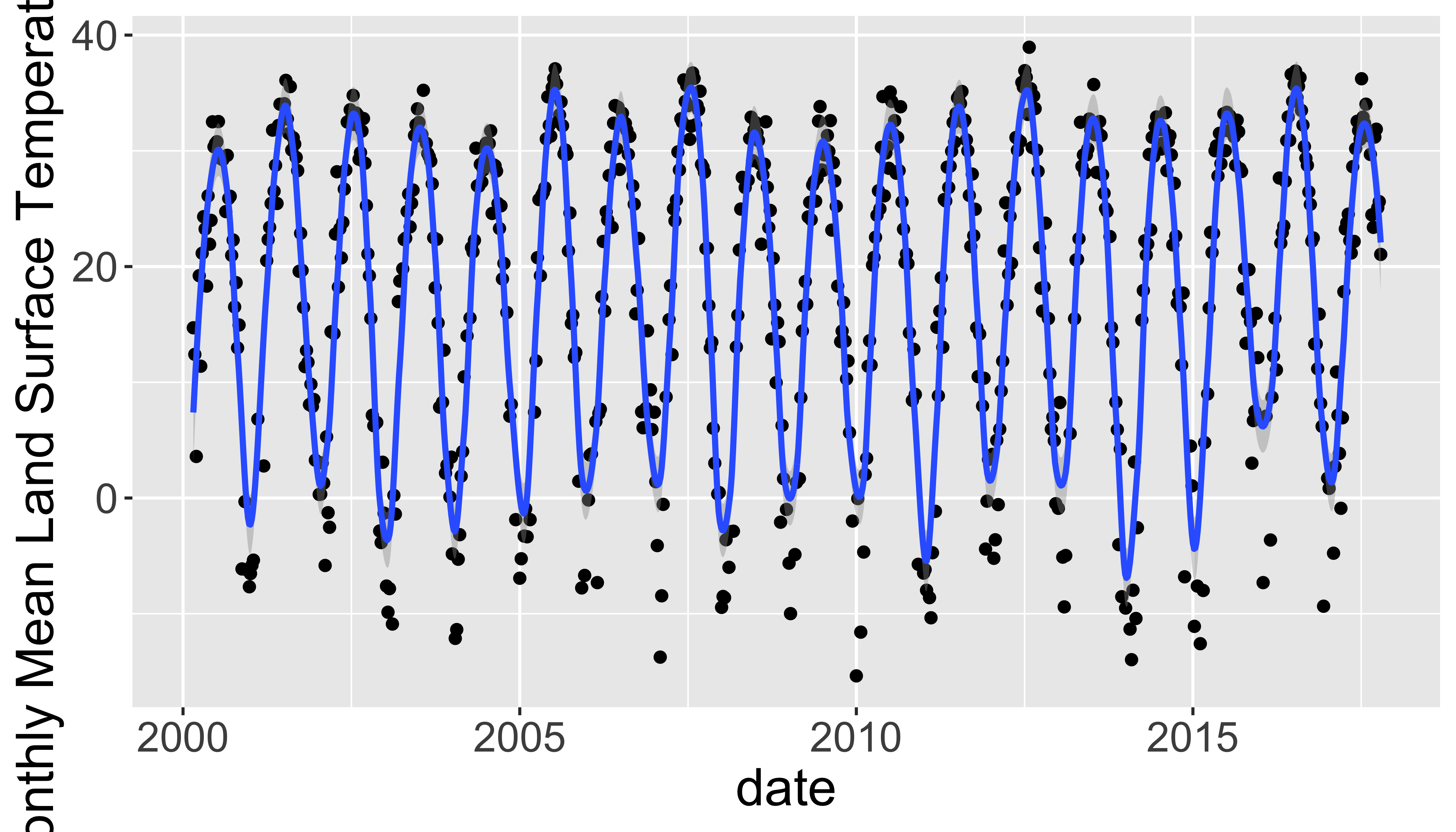
lst=mask(lst,mask=lstkeep,maskval=0)

Add Dates to Z (time) dimension

The default layer names of the LST file include the date as follows:

names(lst)[1:5]

## [1] "X2000.02.18" "X2000.02.26" "X2000.03.05" "X2000.03.13" "X2000.03.21"

Convert those values to a proper R Date format by dropping the “X” and using as.Date().

tdates=names(lst)%>%
  sub(pattern="X",replacement="")%>%
  as.Date("%Y.%m.%d")

names(lst)=1:nlayers(lst)
lst=setZ(lst,tdates)

Part 1: Extract timeseries for a point

Extract LST values for a single point and plot them.

Use lw=SpatialPoints(data.frame(x= -78.791547,y=43.007211)) to define a new Spatial Point at that location.
Set the projection of your point with projection() to "+proj=longlat".
Transform the point to the projection of the raster using spTransform().
Extract the LST data for that location with: extract(lst,lw,buffer=1000,fun=mean,na.rm=T). You may want to transpose them with t() to convert it from a wide matrix to long vector.
Extract the dates for each layer with getZ(lst) and combine them into a data.frame with the transposed raster values. You could use data.frame(), cbind.data.frame() or bind_cols() to do this. The goal is to make a single dataframe with the dates and lst values in columns.
Plot it with ggplot() including points for the raw data and a smooth version as a line. You will probably want to adjust both span and n in geom_smooth.

Your graph should look like this:

See the library(rts) for more timeseries related functions.

Part 2: Summarize weekly data to monthly climatologies

Now we will use a function called stackApply() to calculate monthly mean land surface temperature.

Hints:

First make a variable called tmonth by converting the dates to months using as.numeric(format(getZ(lst),"%m"))
Use stackApply() to summarize the mean value per month (using the tmonth variable you just created) and save the results as lst_month.
Set the names of the layers to months with names(lst_month)=month.name
Plot the map for each month with gplot() in the RasterVis Package.
Calculate the monthly mean for the entire image with cellStats(lst_month,mean)

A plot of the monthly climatologies will look like this:

And the table should be as follows:

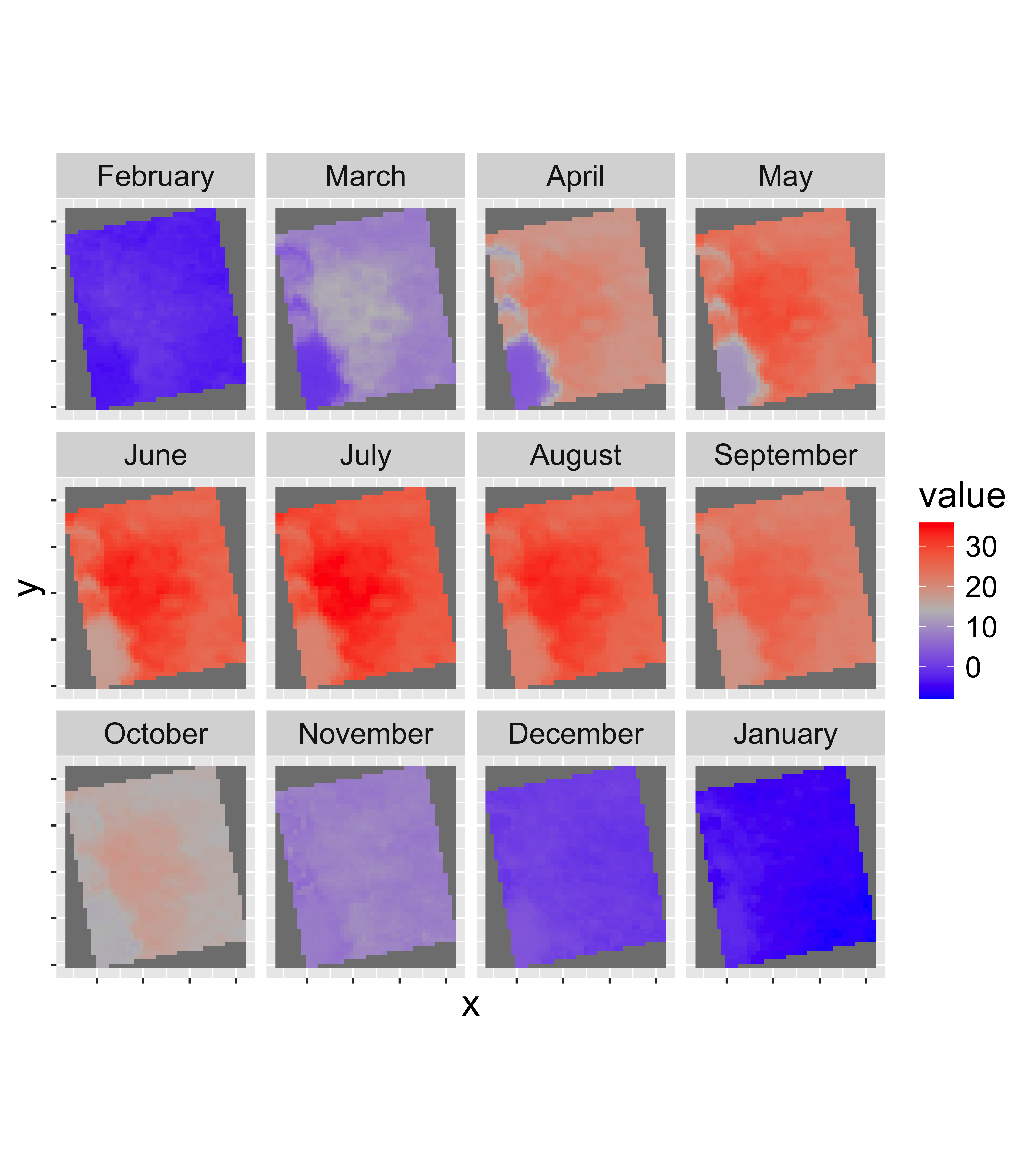
	Mean
January	271.02
February	281.86
March	291.32
April	296.32
May	300.14
June	301.99
July	300.51
August	296.08
September	288.63
October	281.48
November	273.74
December	268.40

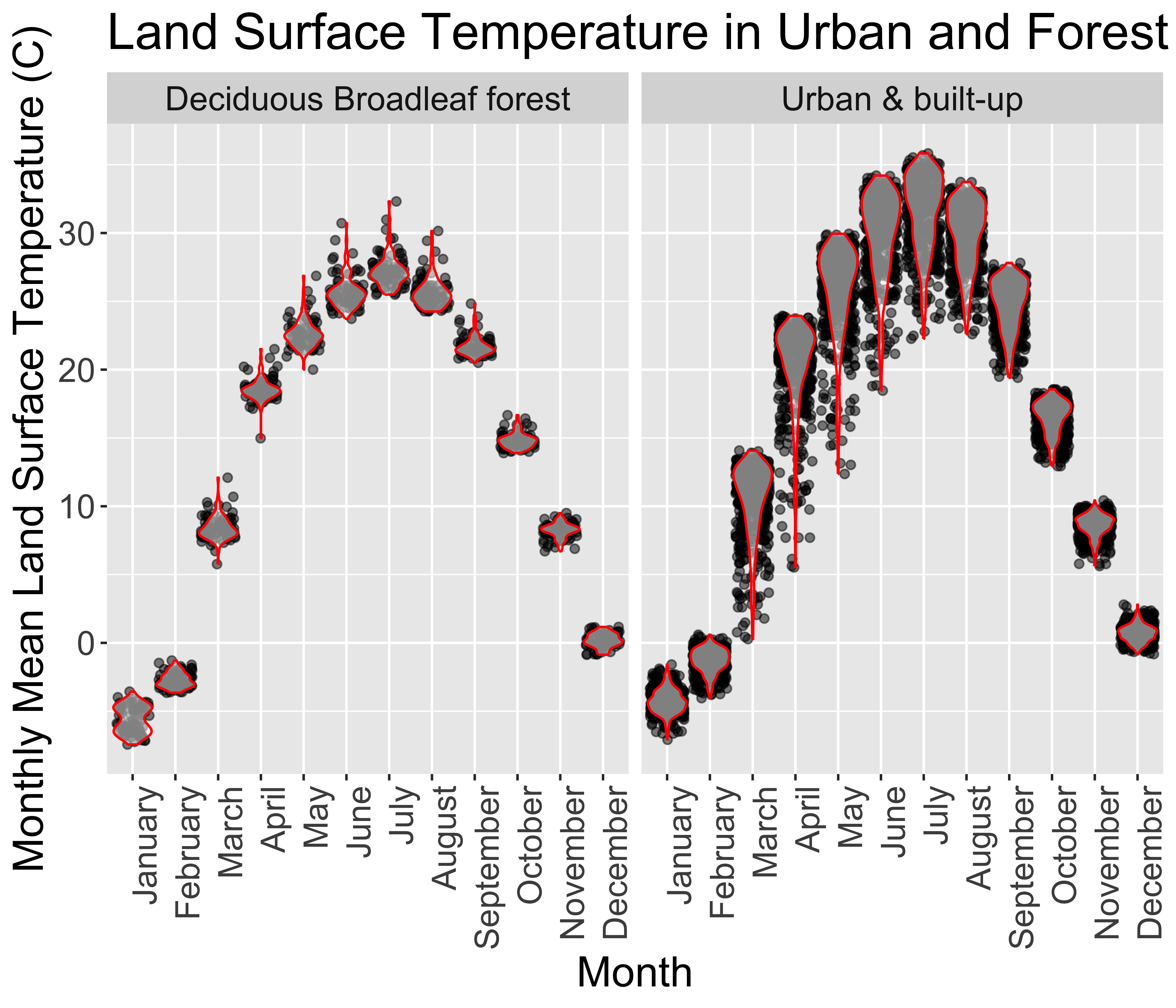
Part 3: Summarize Land Surface Temperature by Land Cover

Make a plot and table to contrast Land Surface Temperature in Urban & built-up and Deciduous Broadleaf forest areas.

Resample lc to lst grid using resample() with method=ngb.

Extract the values from lst_month and lulc2 into a data.frame as follows:

lcds1=cbind.data.frame(
values(lst_month),
ID=values(lulc2[[1]]))%>%
na.omit()

Gather the data into a ‘tidy’ format using gather(key='month',value='value,-ID).
Use mutate() to convert ID to numeric (e.g. ID=as.numeric(ID) and month to an ordered factor with month=factor(month,levels=month.name,ordered=T).
do a left join with the lcd table you created at the beginning.
Use filter() to keep only landcover%in%c("Urban & built-up","Deciduous Broadleaf forest")
Develop a ggplot to illustrate the monthly variability in LST between the two land cover types. The exact form of plot is up to you. Experiment with different geometries, etc.

One potential plot is as follows:

If you have extra time, try to reproduce the table in this box.

This is a more complicated table which involves using the zonal function to aggregate, followed by gathering, spreading, and creative pasteing to combine text fields.

Mean Monthly (±SD) Land Surface Temperature in Buffalo, NY for two landcover classes. Data derived from MODIS LST product (MOD11A2) and MODIS landcover product (MCD12Q1).
month	Deciduous Broadleaf forest	Urban & built-up
January	295.66(±0.92)	299.07(±3.05)
February	294.85(±0.73)	297.98(±1.75)
March	267.47(±1.02)	268.82(±0.85)
April	281.51(±0.84)	283.75(±2.54)
May	270.39(±0.57)	271.89(±0.85)
June	298.71(±1.07)	303.13(±2.29)
July	300.23(±1.11)	304.84(±2.63)
August	291.66(±0.77)	293.51(±3.05)
September	298.7(±1.11)	303.12(±2.93)
October	273.36(±0.56)	273.83(±0.61)
November	281.42(±0.54)	281.78(±0.77)
December	287.9(±0.57)	289.74(±1.15)

Satellite Remote Sensing

Analyze Satellite Data

Tasks

Libraries

Case Study Set up

Identify (and create) download folders

Land Use Land Cover

Load data into R

Explore LULC data

Process landcover data

Land Surface Temperature

Convert LST to Degrees C

MODLAND Quality control

MOD11A2 (Land Surface Temperature) Quality Control

LST QC data

MODIS QC data are Big Endian

Filter the the lst data using the QC data

Select which QC Levels to keep

How many observations will be dropped?

Filter the LST Data keeping only `keepvals`

Add Dates to Z (time) dimension

Part 1: Extract timeseries for a point

Part 2: Summarize weekly data to monthly climatologies

Part 3: Summarize Land Surface Temperature by Land Cover

Satellite Remote Sensing

Analyze Satellite Data

Tasks

Libraries

Case Study Set up

Identify (and create) download folders

Land Use Land Cover

Load data into R

Explore LULC data

Process landcover data

Land Surface Temperature

Convert LST to Degrees C

MODLAND Quality control

MOD11A2 (Land Surface Temperature) Quality Control

LST QC data

MODIS QC data are Big Endian

Filter the the lst data using the QC data

Select which QC Levels to keep

How many observations will be dropped?

Filter the LST Data keeping only keepvals

Add Dates to Z (time) dimension

Part 1: Extract timeseries for a point

Part 2: Summarize weekly data to monthly climatologies

Part 3: Summarize Land Surface Temperature by Land Cover

Filter the LST Data keeping only `keepvals`