Find hottest country on each continent
Use sf and terra to process raster data to quantify mean annual temperature for each country and then identify the hottest one on each continent.
Reading
- Raster Vector Interactions GCR
Background
The raster data format is commonly used for environmental datasets
such as elevation, climate, soil, and land cover. We commonly need to
extract the data from raster objects using simple features
(vector objects). For example if you had a set of points you collected
using a GPS and wanted to know the mean annual temperature at each
point, you might extract the data from each location in a
raster-based map of temperature.
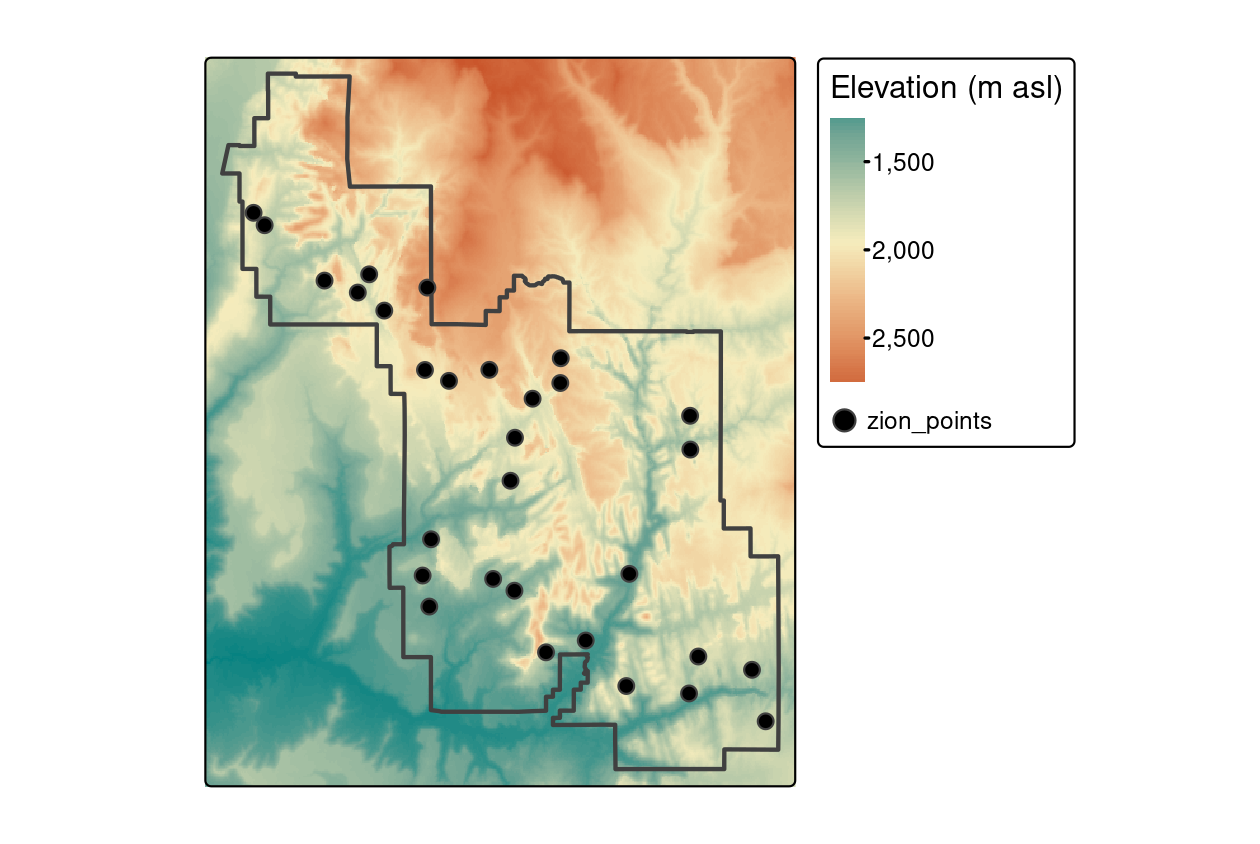
You could also be interested in some summary of the raster data across multiple pixels (such as the buffered points above, a transect, or within a polygon). For example, you might be interested in the mean elevation within the entire polygon in the above figure.
In this case study we’ll work with a HadCRUT temperature data from the Climatic Research Unit at the University of East Anglia. These are near-global rasters of surface temperature on a five degree grid.
Objective
Identify the hottest country on each continent by intersecting a set of polygons with a raster image and calculating the maximum raster value in each polygon.
Tasks
- Calculate annual mean temperatures from a monthly spatio-temporal dataset
- Remove Antarctica from the
worlddataset - Summarize raster values within polygons
- Generate a summary figure and table.
- Save your script as a .R or .Rmd in your course repository
Download starter R script (if desired). Save this directly to your course folder (repository) so you don’t lose track of it!
The details below describe one possible approach.
Libraries
You will need to load the following packages
library(terra)
library(spData)
library(tidyverse)
library(sf)
Loading the spData() package may return a warning:
To access larger datasets...install spDataLarge.... This is
not required - you can use the standard lower resolution files and
safely ignore this message.
Data
Download the mean annual temperatures over the reference period 1961-1990 Climatic Research Unit data (CRU) here. Absolute temperatures for the base period 1961-90 on a 5° by 5° grid. Download these data in netcdf format using the code below:
library(ncdf4)
download.file("https://crudata.uea.ac.uk/cru/data/temperature/absolute.nc","crudata.nc")

# read in the data using the rast() function from the terra package
tmean=rast("crudata.nc")
Note: If the above code returns an error about
nc_open(), try adding method="curl" at the end
of the download.file() command.
Steps
- Prepare Climate Data
- Download and load the CRU data using the code above
(
tmean=rast("crudata.nc")). - Inspect the new
tmeanobject (you can start by just typing it’s nametmean, then perhaps making aplot()). How many layers does it have? What do these represent? You can read more about the data here - The CRU data are stored as degrees C.
- Download and load the CRU data using the code above
(
- Calculate the maximum temperature observed in each country.
- use
max()to calculate the maximum value observed in each pixel across all months. You may want toplot()the output of this and compare the plot of the original (full) raster. How many layers does it have now? - use
terra::extract()to identify the maximum temperature observed in each country (fun=max). Also setna.rm=T, small=Tto 1) handle missing data along coastlines and 2) account for small countries that may not have a pixel centroid in them. - use
bind_cols()to bind the originalworlddataset with the new summary of the temperature data to create a new object calledworld_climwith the outputs from theextract()function above.
- use
- Communicate your results
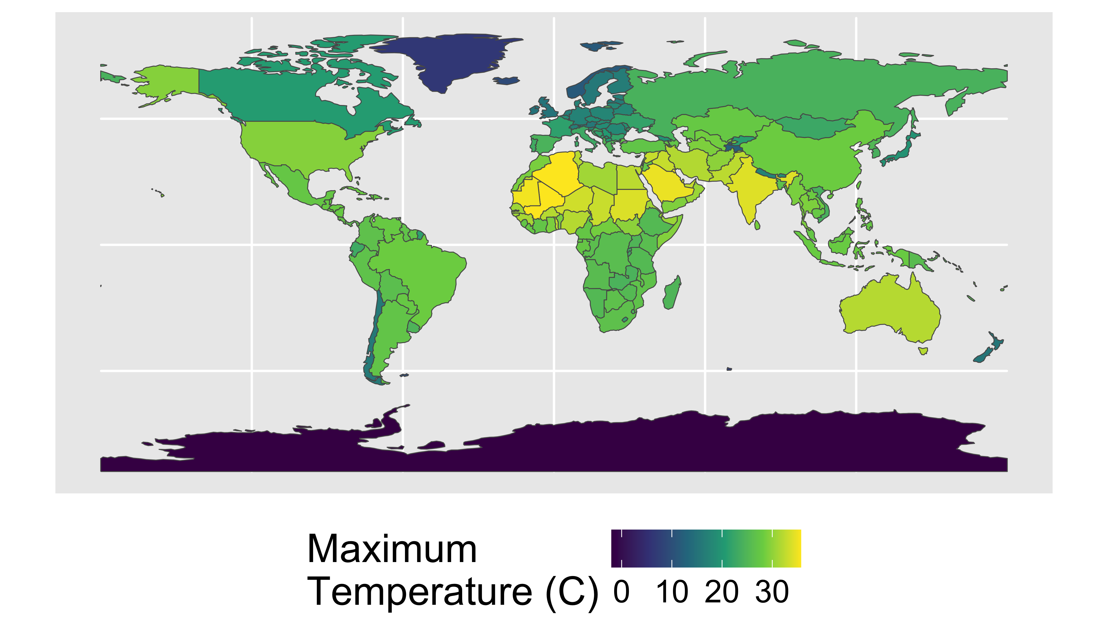
- use
ggplot()andgeom_sf()to plot the maximum temperature in each country polygon (not the original raster layer). To recreate the image below, you will also need+scale_fill_viridis_c(name="Maximum\nTemperature (C)"). Note the use of\nto insert a line break in the text string. You can move the legend around with+theme(legend.position = 'bottom'). - use
dplyrtools to find the hottest country in each continent. You may needgroup_by()andslice_max. To create a nice looking table, you may also want to useselect()to keep only the desired columns,arrange()to sort them,st_set_geometry(NULL)to drop the geometry column (if desired). Save this table ashottest_continents.
- use
Your final result should look something like this:
And the summary table will look like this:
| name_long | continent | max |
|---|---|---|
| Mali | Africa | 35.7 |
| Algeria | Africa | 35.7 |
| Kuwait | Asia | 34.8 |
| Saudi Arabia | Asia | 34.8 |
| Australia | Oceania | 32.0 |
| United States | North America | 29.5 |
| Brazil | South America | 28.2 |
| Albania | Europe | 25.0 |
| French Southern and Antarctic Lands | Seven seas (open ocean) | 7.5 |
| Antarctica | Antarctica | -2.0 |
Note that these data are based on 0.5 degree resolution data and thus will miss small hot places and cannot be directly compared with station-based data.
Build a leaflet map of the same dataset.